
TL;DR
For a graduate BIM course final project, I gave Claude Code plain-English instructions and let it drive Civil 3D, Revit, and Navisworks. Over approximately 32 prompts, it:
- Converted 31 legacy DGN files
- Built the surface, alignment, profile, and corridor for a 2.4-mile road
- Modeled a 716-foot, three-span steel girder bridge in Revit
- Federated all models in Navisworks, flagged a utility clash, and verified zero clashes after revisions
- Plotted the full sheet set
The core work took roughly 3.5 hours: $67 in API tokens plus $875 for my time (billed at a PE’s rate of $250/hour), totaling about $942. By comparison, a skilled Civil 3D drafter would require approximately 290 hours—costing around $32,000 fully burdened.
This process was not hands-off: I caught real errors and exercised all engineering judgment. Much like the steam shovel, AI will not eliminate design work; instead, it shifts daily roles and empowers small teams to execute projects that once required large crews.
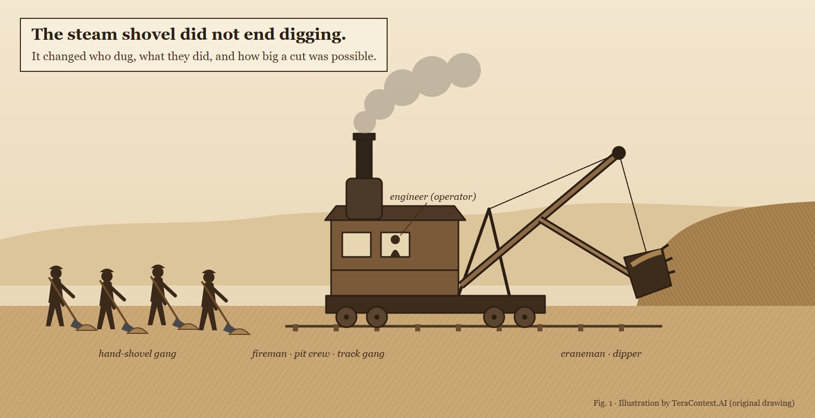 Figure 1. The classic analogy, drawn for this post. The steam shovel replaced the hand-shovel gang, and in doing so it created new jobs: the engineer who ran it, the craneman, the fireman, and the pit crews who moved its track. It also made cuts possible that no affordable gang of shovels could have dug.
The assignment
The project focused on the Berkmar Drive Extension, a real Route 29 Solutions initiative in Albemarle County, Virginia. The design entails a new two-lane urban collector crossing the South Fork Rivanna River via Bridge B-676. The course required a complete federated BIM model including:
- Existing ground surface
- Horizontal and vertical alignments with AASHTO K-value verification
- Assemblies and a roadway corridor
- Stormwater management ponds and a storm sewer network
- A 3D bridge model
- Navisworks clash detection and a 4D construction sequence
- Plotted production sheets
Extra credit tasks required modeling water, gas, electrical, and ITS utilities, as well as detailing the bridge and retaining walls in Revit.
The source deliverables mirrored real-world handoffs: a 298-page roadway plan set, a 71-page bridge plan set, survey data, and 31 MicroStation DGN files—none of which were pre-formatted for the assignment requirements.
I completed the entire project using natural language prompts in Claude Code, an AI agent operating in my terminal. I had previously developed integration bridges for Autodesk products: a command-line driver and an MCP server for Civil 3D, an MCP server for Revit, and a .NET add-in with a command-line runner for Navisworks. Using these tools, Claude read the drawing sets, generated and executed C# and Python scripts against the active applications, inspected the visual outputs, and corrected errors iteratively.
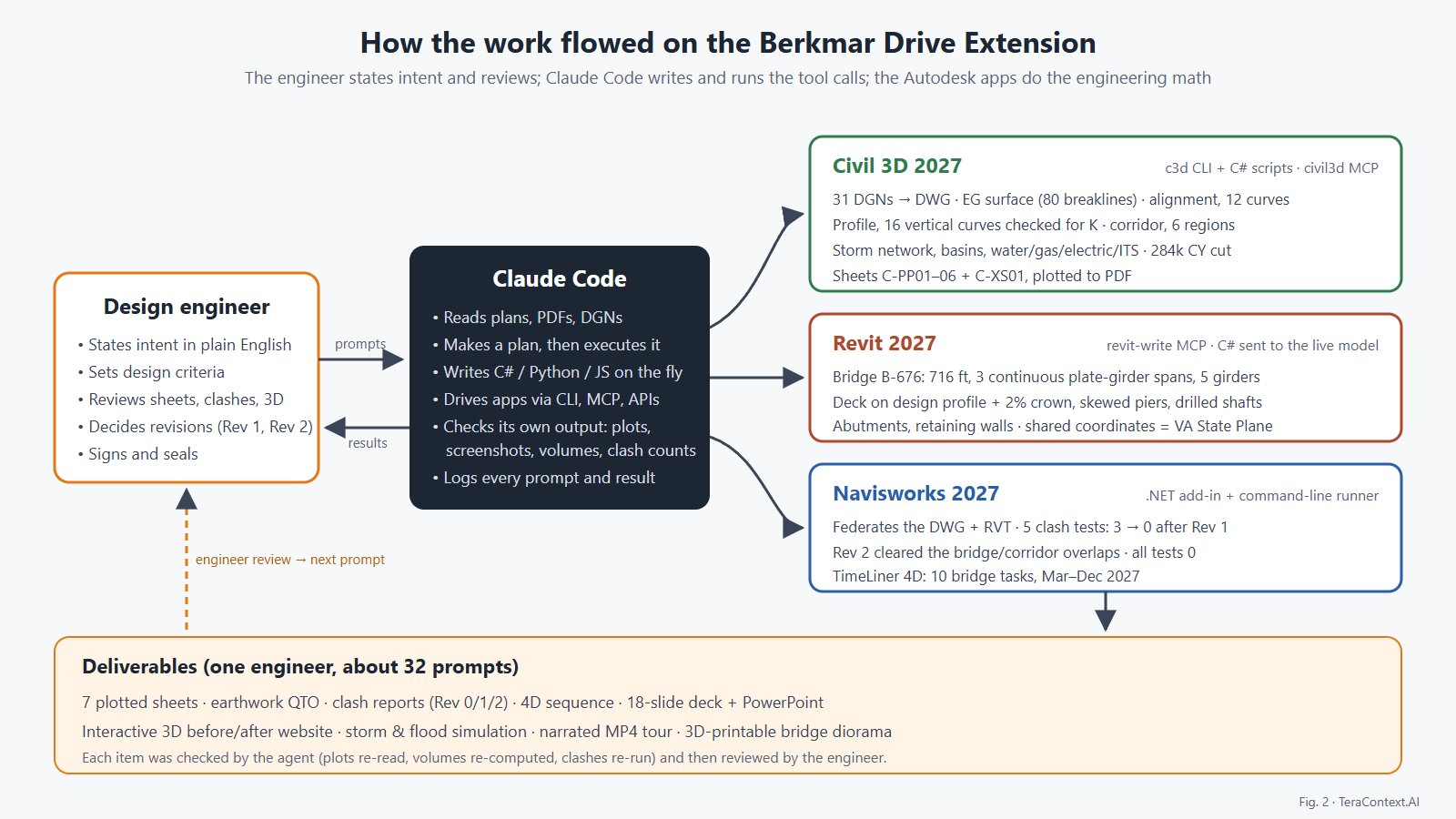 Figure 2. How the work flowed. I stated intent and design criteria and reviewed the output. Claude Code wrote and ran the tool calls. The Autodesk applications did the engineering geometry.
What it actually did
My second prompt was a single detailed paragraph instructing Claude to analyze all files, take an inventory, attempt the extra credit, model the bridge in Revit, formulate an execution plan, and run autonomously while I stepped away.
Over the subsequent sessions, Claude executed the work step by step:
- Reading the plans. Because the plan PDFs were vector drawings without selectable text, Claude rendered them as images for visual inspection. It successfully extracted the index of sheets, alignment data for 12 horizontal curves with PI coordinates, typical cross-sections (11-foot lanes, bike lanes, curb and gutter, a sidewalk on one side, and a shared-use path on the other), and the bridge general plan.
- Converting the DGNs. Claude determined the exact command sequence for Civil 3D’s DGN import process, handling edge cases such as models storing data within
Seed2Dspaces. It batch-converted all 31 files and verified their overlay alignment in the Virginia State Plane South coordinate system. - Civil 3D model.
- Existing Ground: Generated a surface utilizing 80 breaklines.
- Alignment: Reconstructed the horizontal alignment directly from curve tables.
- Profile: Built a design profile with 16 vertical curves, confirming all met AASHTO minimum K-values for 40 mph.
- Corridor: Created a roadway corridor across six regions and three assemblies, leaving an intentional gap for the bridge structure.
- Earthwork: Calculated approximately 284,000 cubic yards of cut and 220,000 cubic yards of fill, validating the end-area volumes against a TIN-to-TIN surface comparison.
- Plan and profile sheets. Claude generated PDF sheet plots and visually inspected its own output by reading the rendered PDFs back into context. This feedback loop proved critical: it caught station labels that stopped rendering following a corridor rebuild, resolved overlapping text, and restored a missing north arrow—fixing these issues autonomously before review.
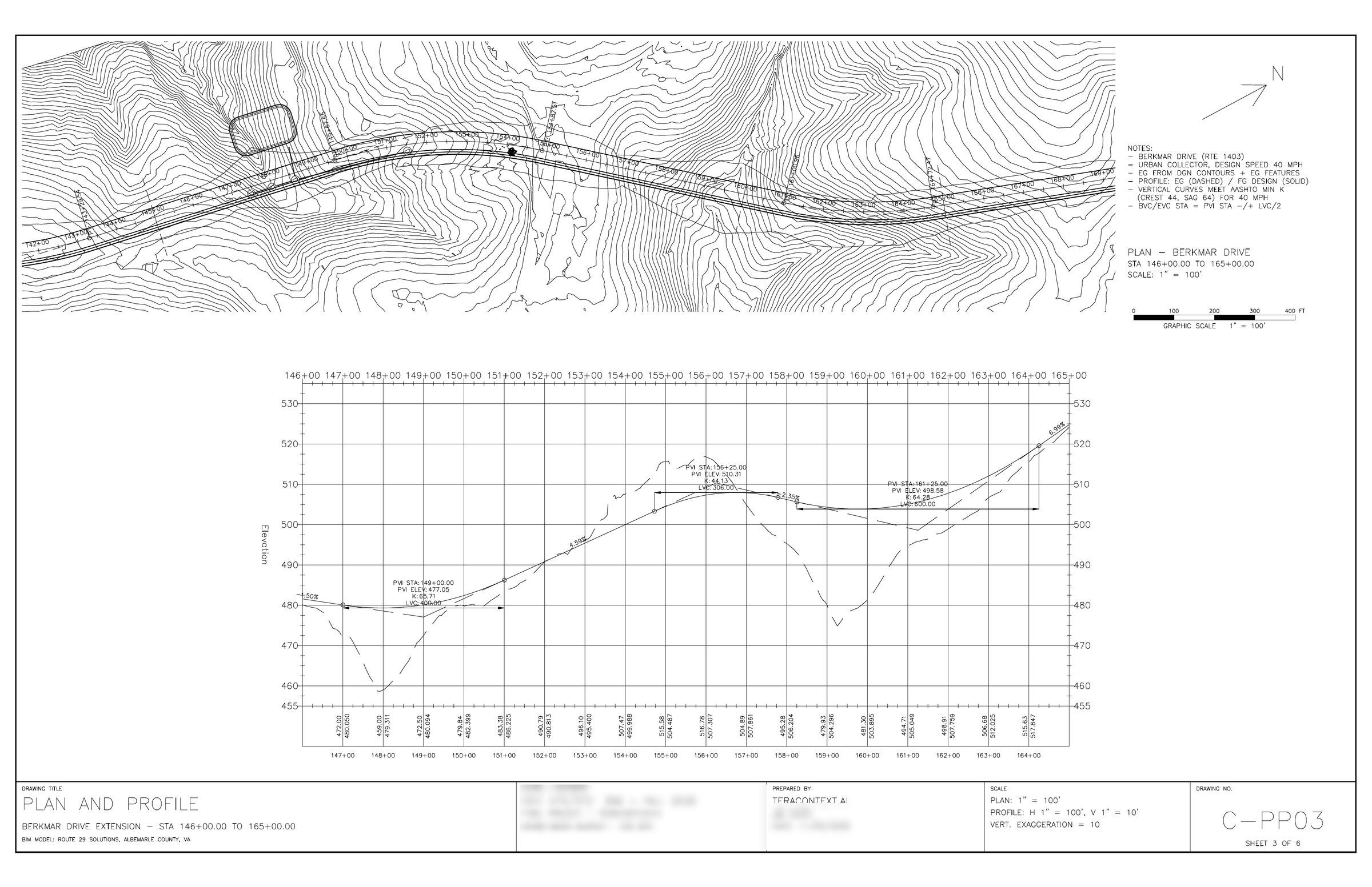 Figure 3. Sheet C-PP03, plotted from the Civil 3D model. The plan is on top (contours, alignment, Bioretention Basin #1) and the profile below, with the dashed existing ground, the solid design grade and the vertical-curve data. Claude checked every sheet by reading back its own plots.
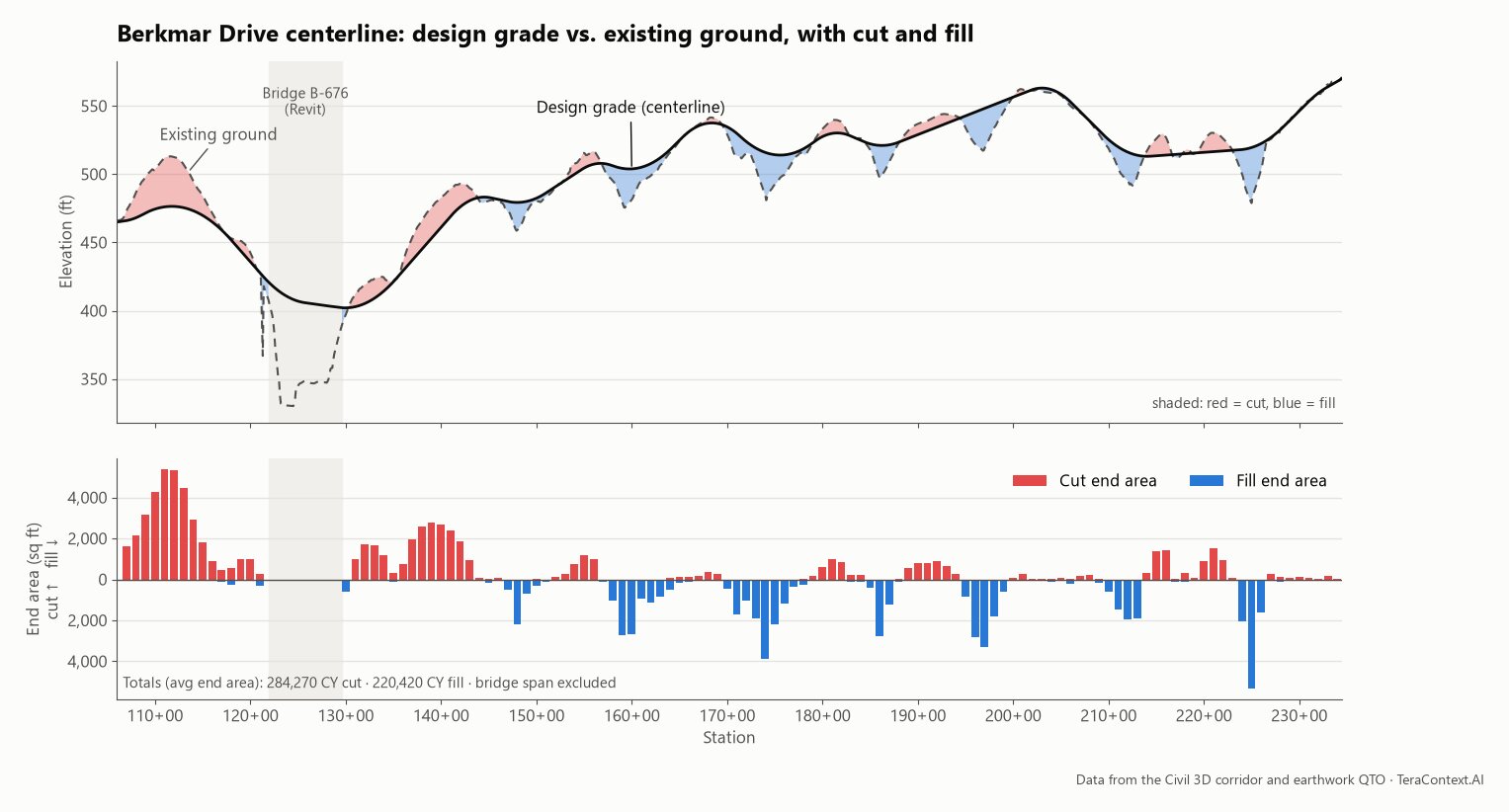 Figure 4. The centerline design. The top panel shows the design grade (solid) over the existing ground (dashed) along the 2.4-mile alignment, with cut shaded red and fill shaded blue. The gray band is the river crossing, where the road is carried by the bridge instead of earthwork. The bottom panel shows the cut and fill end areas every 100 feet, the raw material for the 284,000 CY of cut and 220,000 CY of fill. Most of the cut is in the hill south of the river, and the fills are scattered across the stream valleys to the north.
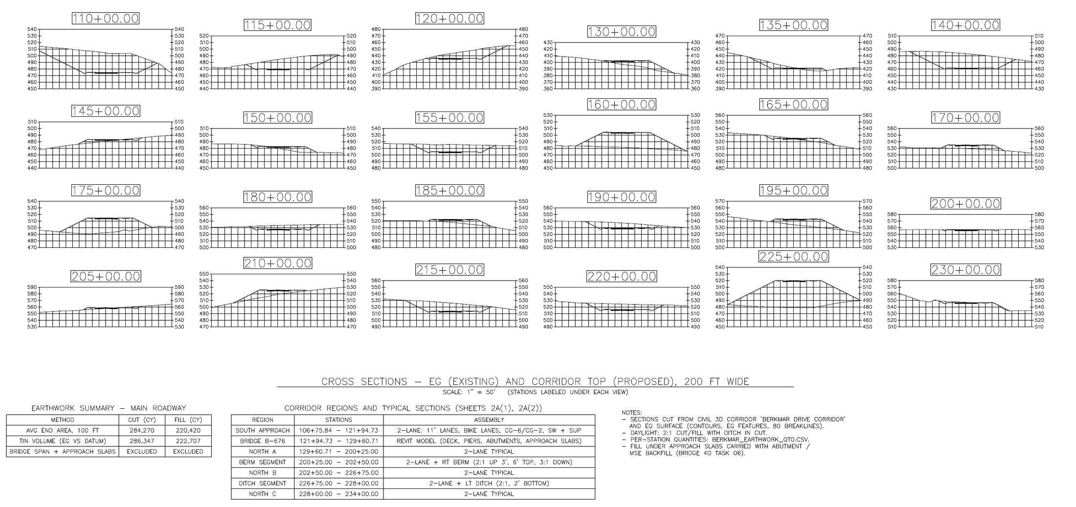 Figure 5. Sheet C-XS01: road cross-sections every 500 feet, cut from the corridor against existing ground. Each one shows the 2-lane typical section, with 2:1 daylight slopes to the ground and a ditch in cut. Below them are the earthwork summary (average-end-area checked against a TIN-to-TIN volume) and the six corridor regions with their assemblies.
- The bridge in Revit. Claude issued C# scripts to the active Revit session to construct Bridge B-676 based on the bridge plan set:
- Three continuous steel plate-girder spans (276 ft, 211 ft, and 225 ft)
- Five plate girders supporting a deck matching the roadway profile and 2% cross-slope
- Skewed pier caps resting on drilled shafts, along with abutments and retaining walls
By sharing coordinate definitions with the Civil 3D model, the Revit assembly aligned seamlessly with state plane coordinates without requiring manual positioning.
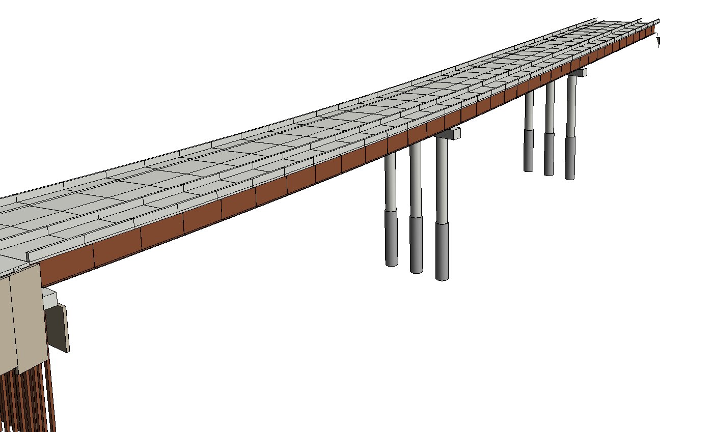 Figure 6. Bridge B-676 in Revit: the deck following the vertical curve, the plate girders, two skewed piers on drilled shafts, and the south abutment with its piles in the foreground.
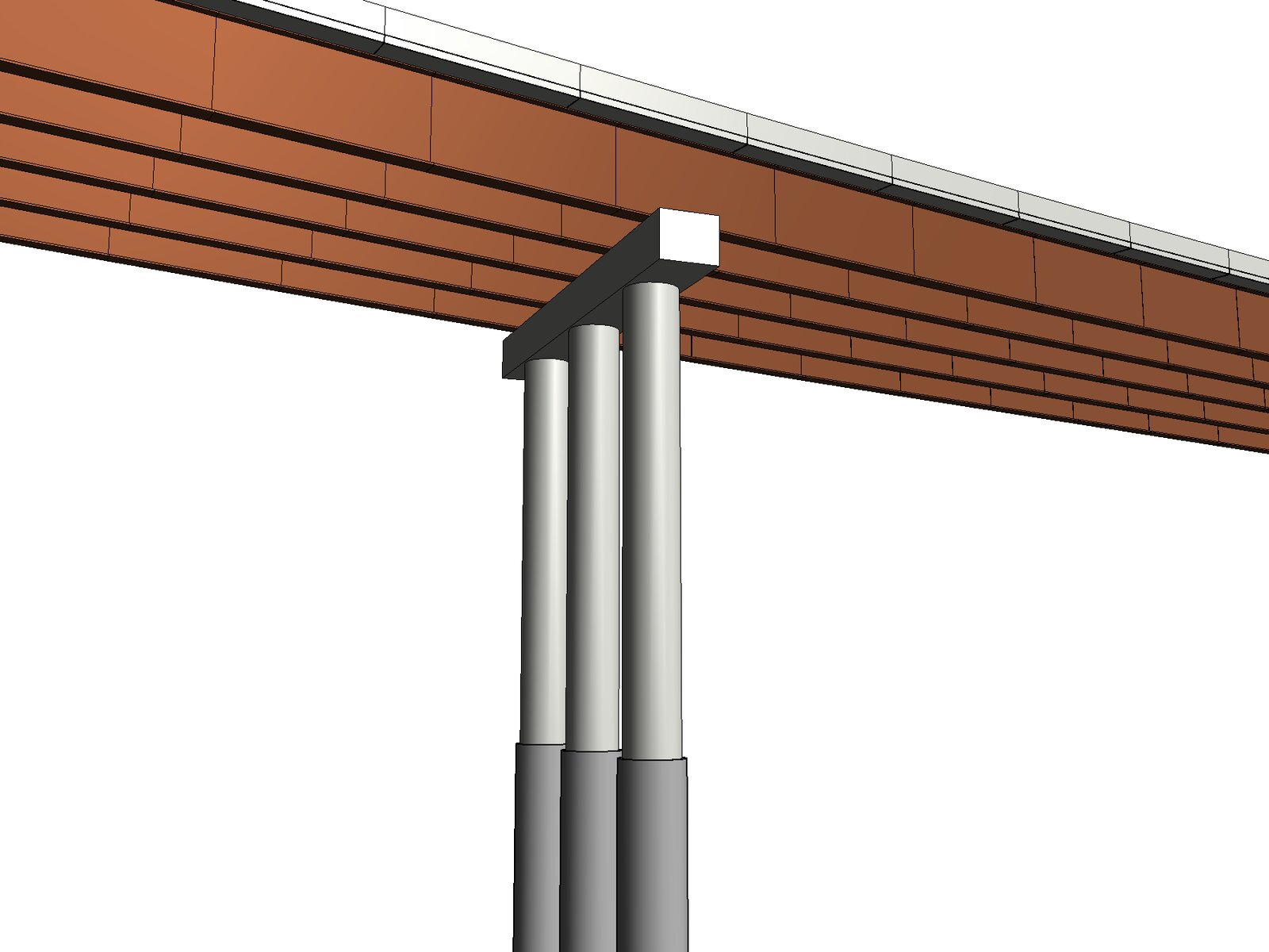 Figure 7. Bridge B-676 in Revit, looking up at a pier: plate girders, the pier cap, and three columns on drilled shafts. The model was built entirely from C# that Claude wrote and sent into the live Revit session.
- Navisworks. Claude federated the Civil 3D roadway drawing and Revit bridge model, configuring five distinct clash detection tests.
- Initial Clash: The first run identified an interference where storm pipe 10-3 to 10-4 intersected the ITS and electrical duct banks.
- Revision 1: When asked if lowering the utility duct banks would resolve the conflict, Claude modified the elevations in Civil 3D, re-exported the model, and re-ran clash detection to confirm zero remaining interferences.
- Revision 2: Nine residual bridge-versus-corridor overlaps were identified as a redundant corridor region. Once removed in Revision 2, all clash tests passed cleanly.
Claude also constructed a 4D TimeLiner sequence mapping out ten major bridge construction phases scheduled from March to December 2027.
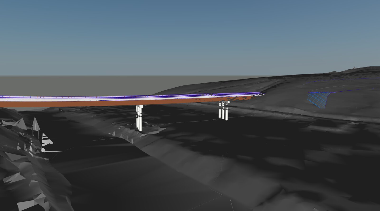 Figure 8. The federated model in Navisworks: the Revit bridge over the Civil 3D surfaces and corridor, with five clash tests run against it.
Once core project requirements were completed, I requested an interactive 3D site website comparing “before” and “after” conditions. Claude built the application using Three.js and hosted it locally via Caddy. Features included:
- Public high-resolution aerial orthophotos from Virginia’s GIS database (2013 flights for “before” conditions and the latest flight for “after”)
- Approximately 28,000 trees, river geometry, animated traffic, and a first-person drive mode
- A storm simulation engine raising river levels to the design flood stage to verify bridge clearance and model bioretention basin filling
- A narrated cinematic video tour featuring synthetic voice narration generated by a local text-to-speech model
Additionally, Claude prepared a 3D-printable diorama file of the bridge tailored for a desktop 3D printer.
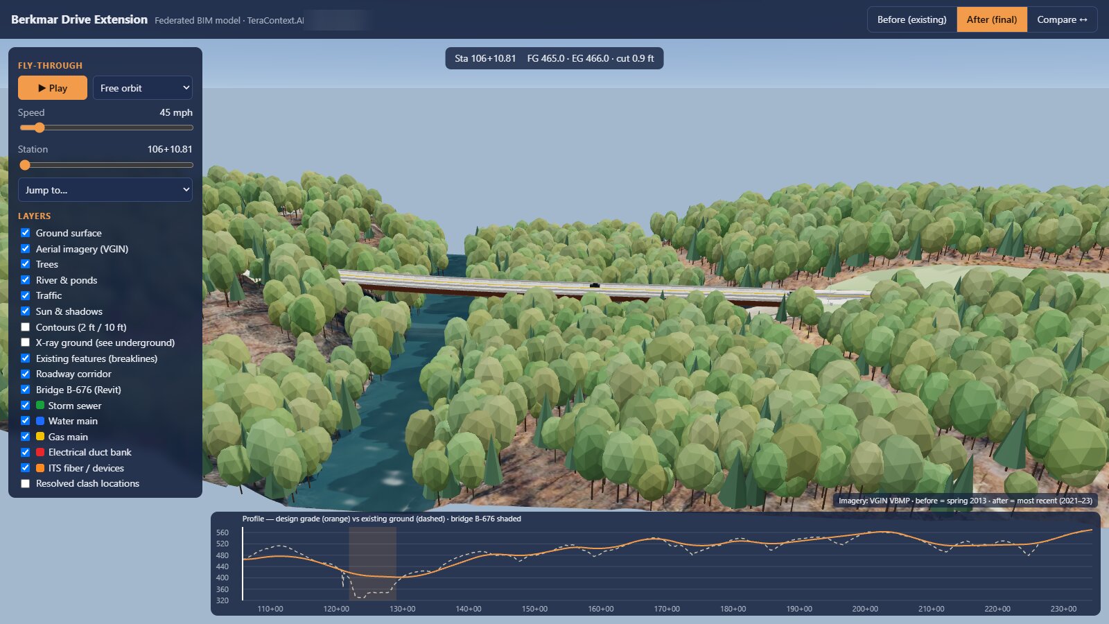 Figure 9. The aerial imagery draped on the 3D terrain. The orthophoto is draped over the existing-ground surface, with the corridor, the Revit bridge, the river and the trees placed on it, all in the same state plane coordinates as the Civil 3D model. The readout at the top shows finished grade, existing ground and cut depth at the current station. The strip at the bottom is the same profile as Figure 4.
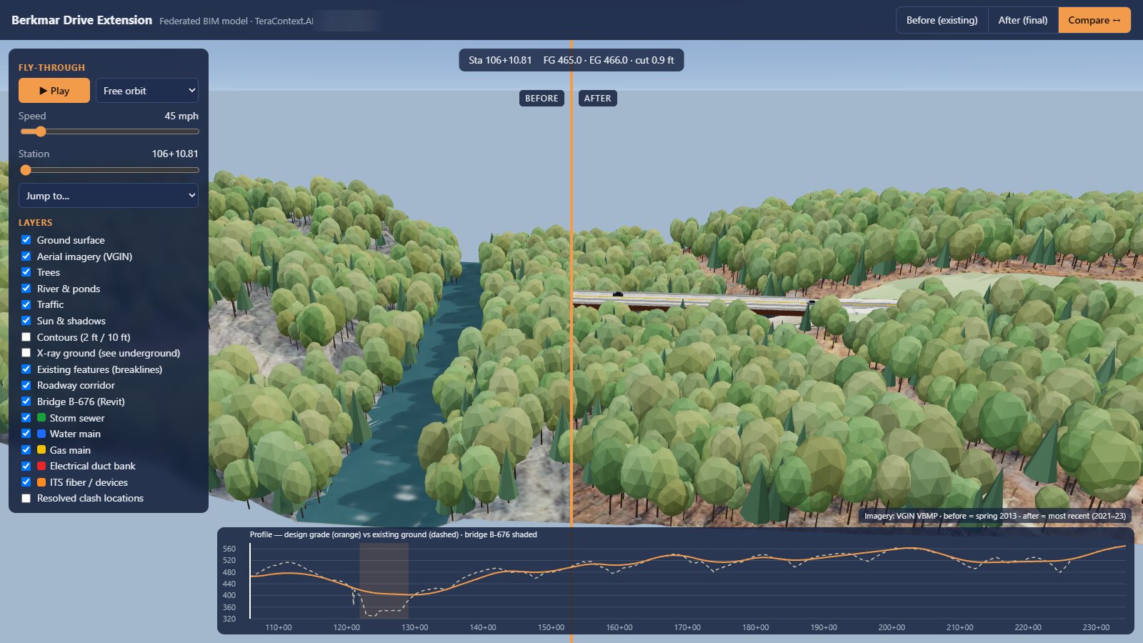 Figure 10. The interactive website: the 2013 forested valley on the left of the divider, the finished design with Bridge B-676 on the right, and the design profile along the bottom. This was not required by the assignment. It exists because it was cheap to ask for.
The narrated cinematic tour (1 minute 46 seconds): the 2.4-mile alignment, the finished design, the 4D bridge sequence, a storm filling Bioretention Basin #1, and a drive along the new road. The narration was generated by a local text-to-speech model.
What it got wrong (and why that matters)
Presenting this workflow as fully push-button automation would be inaccurate. That reality is why the cost evaluation explicitly accounts for my time billed at a Professional Engineer’s (PE) rate. A licensed engineer must actively direct the process—monitoring outputs, flagging agent oversights, and making final design decisions.
Several software and execution issues occurred during the run:
- Civil 3D froze completely, requiring a system reboot.
- A Revit export routine crashed the host application.
- Scripting queries against a specific Civil 3D object caused two application crashes.
- Corridor rebuilds occasionally caused station labels to disappear.
- The initial drive-through camera was positioned in the oncoming lane facing traffic, and a subsequent video render suffered GPU encoding corruption during a scene transition.
Two distinct operational patterns emerged from these failure modes:
- The agent resolved most errors when granted visual feedback. By reviewing rendered plots, auditing clash counts, verifying volumes, and evaluating viewport screenshots, the agent self-corrected. Multimodal tools that let an agent inspect its output fundamentally change performance compared to headless code execution.
- Human oversight caught higher-level anomalies. Visual flaws—such as the inverted drive direction or video artifacting—were immediately apparent upon human review. One-sentence feedback (“it looks like you are driving on the left side of the road”) enabled Claude to diagnose root causes—such as a sign error in the offset vector or GPU memory contention—and apply fixes quickly.
Crucially, core engineering decisions remained human-driven: selecting whether to lower duct banks versus rerouting storm lines, establishing design flood criteria, and evaluating slope or clearance trade-offs. Claude analyzed options and outlined trade-offs, but executed changes only upon explicit approval.
The steam shovel
I previously introduced this analogy in The Steam Shovel Moment for Civil Engineering Drafting (October 8, 2026) regarding AI agents generating individual Civil 3D drawings. The comparison warrants repeating here because it scales directly to full project workflows: from initial survey data to final sheet sets across three design platforms, complete with revisions and clash reports.
Prior to mechanized excavation, major earthwork required large crews using hand shovels and wheelbarrows. William Otis patented the steam shovel in 1839, and by the late 19th century, rail-mounted shovels dominated railway and canal construction. A single machine could easily outperform dozens of laborers, prompting early fears of widespread worker disemployment.
In practice, labor dynamics evolved rather than vanished. Operating each shovel required a skilled operator, a craneman to handle the dipper, a fireman to maintain boiler pressure, and pit crews to continuously lay track sections. Additional crews operated spoil trains, while mechanics maintained the fleet. Labor shifted from manual excavation to operating, maintaining, and logistics management around machinery.
Crucially, steam shovels enabled infrastructure projects that were previously infeasible due to labor and cost constraints. The construction of the Panama Canal illustrates this shift. The French attempt in the 1880s had steam shovels too, but disease, mudslides, and financial collapse halted the work. The American project (1904–1914) scaled mechanized operations dramatically:
- Deploying 102 steam shovels, 77 of them 95-ton Bucyrus models with five-cubic-yard dippers
- Rebuilding the railroad so spoil trains ran continuously on double track; on a typical day, about 160 trainloads of material left the Culebra Cut
- Setting excavation records, such as a single Bucyrus shovel moving 70,000 cubic yards in 26 days in March 1910
Despite extensive mechanization, the project employed nearly 40,000 workers at its 1913 peak and over 56,000 people across the decade. While public health interventions—such as William Gorgas’s sanitation and mosquito-control campaign—were essential to keeping workers alive, the physical excavation of the Culebra Cut would have been impossible without heavy steam equipment and rail infrastructure.
The steam shovel did not shrink the construction industry; it expanded the scale of what could be built while transforming workforce roles. AI agents driving engineering software represent a similar inflection point for infrastructure design.
The arithmetic: one agent versus one drafter
The relevant benchmark for AI design agents is not a licensed engineer. A software agent cannot sit for a PE exam or stamp engineering plans, nor does a senior engineer typically execute baseline CAD drafting. In traditional workflows, a PE assigns production work to an experienced CAD technician, reviews the submittals, and issues redlines. The agent effectively replaces the drafting role, while the required engineering review time remains identical in both approaches.
For the core scope—the required civil model and Revit bridge details, excluding the web application, video, and 3D print—the agent completed the workload in 3.5 hours of wall-clock time and ~$67 in API tokens. The table below outlines an estimated breakdown for an experienced CAD drafter performing the same tasks from raw PDFs and DGN files:
| Task | Drafter hours |
|---|---|
| Project setup, standards, templates, and coordinate system definition | 16 |
| DGN file conversion and georeferencing (31 files) | 16 |
| Existing-ground surface generation (80 breaklines) | 12 |
| Horizontal alignment (12 curves) and design profile (16 vertical curves with K-value checks) | 20 |
| Assemblies, six-region corridor modeling, and earthwork quantity extraction | 30 |
| Storm sewer network and bioretention basin design | 24 |
| Utility network modeling (water, gas, electric, ITS) | 24 |
| Seven production plan-and-profile sheets with annotations | 24 |
| Revit bridge modeling: girders, deck profile, skewed piers, and drilled shafts | 60 |
| Abutments and retaining wall modeling | 16 |
| Navisworks federation, five clash detection setups, and reporting | 16 |
| 4D TimeLiner construction sequence setup | 12 |
| Two revision cycles across models, clash sets, and sheet sets | 16 |
| Total | ≈ 290 |
This scope corresponds to roughly seven full workweeks (~290 hours), with typical industry ranges spanning 250 to 350 hours depending on team specialization.
A senior civil drafter earns roughly $35–$40 per hour in wages. Applying a standard consulting-firm multiplier of 2.5× to 3.0× (benefits, payroll taxes, office, software licenses, overhead, and profit) yields a fully burdened rate of about $110 per hour. At $110/hour, 290 hours equals approximately $32,000 (ranging between $25,000 and $40,000).
Deploying an agent requires an operator to direct prompting and review outputs. Accounting for 3.5 hours of senior engineer oversight at a fully loaded PE billing rate of $250/hour ($875 total labor) alongside $67 in API tokens yields a total cost of ~$942. Token consumption accounts for only about 7% of the total expense, meaning engineer time remains the primary cost driver.
| Metric | Agent + PE operator | Skilled drafter |
|---|---|---|
| Time | ~3.5 hours | ~290 hours (~7 weeks) |
| Tokens | ~$67 | — |
| Labor | ~$875 (PE, 3.5 h × $250) | ~$32,000 (290 h × $110) |
| Total | ~$942 | ~$32,000 |
| Ratio | — | ~80× the time, ~34× the cost |
Key context for these comparisons:
- Review Overhead: Standard PE markup and QA/QC review time is excluded from both models as it remains constant regardless of production method.
- Tooling Investment: The agent estimate excludes prior development time spent creating the CLI and MCP API bridges.
- Model Maturity: The human drafter estimate assumes full production-level deliverables, whereas the agent output represents a detailed academic student model.
Even under conservative assumptions—paying senior PE rates for all operator time and halving estimated efficiency gains—the agent-assisted workflow delivers the scope at less than one-tenth the cost in a single afternoon rather than two months. When design production costs drop dramatically, engineering volume scales accordingly.
How the daily work of a design engineer changes
Based on this workflow, several clear shifts emerge for engineering practice:
The engineer becomes the machine operator, not the excavation gang. A significant portion of entry-level engineering work currently involves mechanical CAD tasks:
- Converting file formats across legacy systems
- Configuring label styles and display properties
- Constructing corridors region by region
- Updating plan sheets after minor design edits
- Re-running clash detection scripts and documenting findings
These repetitive actions represent hand-shovel labor—the exact tasks automated most effectively by the agent. The engineer’s role pivots to defining project intent, establishing design criteria, reviewing results, and making final engineering determinations.
Rigorous technical review becomes the core skill. When generating complex plan sets requires minimal prompt effort, technical verification becomes the primary operational bottleneck. Engineers will allocate more time to QA/QC review rather than manual drafting:
- Evaluating centerline profiles for improper grades or drainage issues
- Identifying visual inconsistencies in renderings and 3D perspectives
- Assessing whether minor geometric overlaps warrant design modifications
This shift elevates the importance of an experienced engineering eye. It also raises an essential question for firm leadership: how will junior engineers develop deep intuition when routine drafting work is automated? The traditional apprenticeship model—where young engineers master design details through repetitive production work—must be intentionally redesigned.
Low-cost iteration improves overall design quality. Executing design revisions required simple prompts that automatically propagated changes across Civil 3D models, Revit structures, Navisworks clash sets, and sheet sets. Rapid iteration enables engineering teams to evaluate broader design alternatives:
- Testing multiple horizontal and vertical alignments simultaneously
- Re-evaluating storm sewer capacity against extreme flood scenarios after every change
- Generating 4D construction sequences for minor structures that previously lacked budget for complex scheduling
- Delivering interactive 3D fly-throughs for public outreach on standard projects
Rather than eliminating roles, affordable iteration enables deeper engineering rigor and scope expansion that project budgets previously precluded.
New specialized roles emerge around AI toolchains. This project relied on specialized integrations connecting Claude Code to Autodesk APIs (via custom CLI drivers, MCP servers, and Navisworks add-ins). Firms adopting agentic workflows will require dedicated roles to:
- Translate firm CAD/BIM standards into machine-readable prompts and configuration rules
- Maintain audit trails and decision logs (such as the 32-prompt log maintained for this project)
- Define governance frameworks governing autonomous execution boundaries
- Provide professional licensure oversight and sign-off on AI-assisted deliverables
These technical and governance roles represent the modern equivalents of crane operators, firemen, and pit crews.
Small teams gain the capacity of large engineering firms. While the Berkmar Drive Extension project yielded an academic BIM model rather than final construction drawings, a single engineer generated a multi-application BIM model, complete sheet set, and web visualization in a handful of working sessions. Armed with agentic workflows, a small firm can compete for infrastructure scope that historically required substantial drafting departments, enabling public agencies and mid-sized firms to tackle project backlogs more aggressively.
Unemployment, or a bigger canal?
Concerns regarding displacement are understandable: if an agent allows one engineer to produce the work of ten, will firm headcounts drop by 90%? Historical precedents suggest otherwise. Infrastructure demand has rarely been constrained by a lack of societal need; rather, it is capped by the economic cost of engineering and construction labor.
Modern communities face severe infrastructure deficits: aging bridges, stormwater systems unequipped for changing climate patterns, and municipal transportation corridors stalled in planning phases for decades. Dramatically reducing design costs expands the volume of economically viable infrastructure projects.
Daily engineering roles will inevitably transform. Manual DGN conversions and repetitive label formatting will give way to decision-making, quality verification, interdisciplinary coordination, and public engagement, alongside new technical roles focused on AI system architecture and governance.
Firms and practitioners who adapt to these tools will expand their capabilities. Those who resist technological shifts will face challenges, echoing the transition experienced by manual excavation crews in the 19th century.
Reflecting on this project, the most striking takeaway was not merely execution speed, but project scope. Lowering the cost of iteration made ambitious deliverables feasible that would otherwise have been discarded due to time constraints.
The canal simply got bigger.
Built with Claude Code (Opus 5.5) driving Civil 3D 2027, Revit 2027, and Navisworks 2027 through custom CLI, MCP, and API bridges.
Sources for the history
- TeraContext.AI, The Steam Shovel Moment for Civil Engineering Drafting (October 8, 2026), the earlier post this one builds on.
- Panama Canal Authority, construction workforce by year (peak 39,962 in August 1913) and Canal FAQ (56,307 employed, 1904–1913).
- Smithsonian Libraries, Make the Dirt Fly! (102 steam shovels, most built by Bucyrus; the largest 95 tons with five-cubic-yard dippers).
- Wikipedia, Culebra Cut and Bucyrus-Erie (160 trainloads a day; 77 of the 102 shovels were Bucyrus; the March 1910 output record; the May 1913 breakthrough).
- PBS American Experience, TR’s Panama (the French effort, Stevens’s continuous double-track spoil trains, Gorgas and sanitation).
- Smithsonian Magazine, How the Panama Canal took a huge toll on the contract workers who built it (workforce origins).
- Transportation History, 1839: William Otis’s steam shovel patent.


