In Steam Shovels for Design Engineers, Claude Code drove three Autodesk applications through a graduate BIM course project, the Berkmar Drive Extension in Albemarle County, Virginia. It produced:

the Civil 3D corridor and sheets;
a Revit model of Bridge B-676, a 716-foot, three-span steel plate-girder bridge over the South Fork Rivanna River;
a federated Navisworks model with clash detection.

The steam-shovel point was about drafting: the digging got faster, but someone still had to decide where to dig.

This post takes the same bridge somewhere drafting never goes: into physics. Over one long working session, Claude Code drove the open-source finite-element package Elmer FEM from the command line. It set up, ran, debugged and checked:

a transient heat analysis of the deck through a hot July day, with the real sun path and the shadows of the parapets;
a 3D structural model of the whole superstructure, with a 10° skew and 44 lines of cross-frames, under construction-stage dead load, shrinkage, design temperature gradients, the simulated sunny day, a sweep of HL-93 trucks, and free vibration;
an AASHTO LRFD strength, service, constructibility and fatigue check of the girders, which then resized the flange plates until every check passed.

The headline isn’t any single number. It’s the shape of the workflow:

the agent did the heavy lifting of meshing, input files, runs, post-processing and plots;
every result was checked against an independent calculation;
those checks caught eleven errors that produced plausible-looking answers.

That last part is the real story, and it’s why the engineer’s time still belongs in the budget.

Disclaimer: for demonstration and education only. Every simulation, number, code check and plate size in this post was produced to demonstrate a workflow. None of it is engineering work stamped or sealed by a licensed Professional Engineer, none of it has been independently reviewed, and none of it should be used to design, build, rate or evaluate a real structure. The bridge geometry is the one built for the BIM model, the material properties are assumed typical values, and the girder sizes in the Revit model were placeholders. As you’ll see, the code check makes that clear.

The bridge

B-676 carries a two-lane urban collector over the South Fork Rivanna River in central Virginia:

Spans: three continuous spans of 270, 211 and 220 ft between bearings, as modeled.
Girders: five 110-inch-deep weathering-steel plate girders at 11′-7″ spacing.
Deck: a 9.5-inch concrete deck on a 2% crown.
Across the deck: a raised 6-ft sidewalk on the north-west side, a 30-ft roadway, a median rail, and a 14-ft shared-use path on the south-east side.
Barriers: BR27C concrete parapets on both edges.
Orientation: the bridge axis runs N 40.9° E, a detail that matters once the sun comes up.
Supports: on a 10° skew.

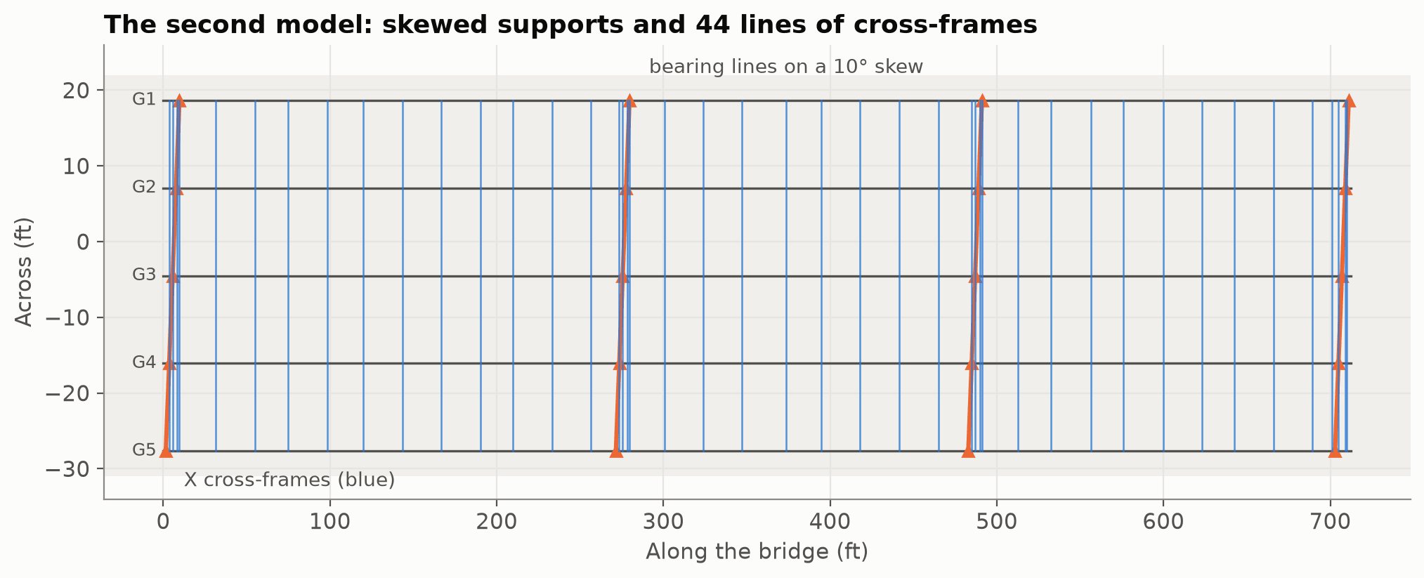Figure 1. Plan of the 3D model: five girders, bearing lines on a 10° skew (orange), and the X cross-frames between the girders (blue).

None of the material properties were specified, so the analysis uses typical values, all documented in the study:

Concrete: f′c = 4 ksi, and Ec = 3,990 ksi per AASHTO 5.4.2.4. Superimposed dead load and shrinkage use Ec/3, which represents creep.
Steel: A709 Grade 50W.
Superimposed loads: a 25 psf future wearing surface, and the AASHTO 75 psf pedestrian load on the sidewalk and path.
Thermal gradient: the AASHTO zone 2 design gradient, the worse of the two zones that could apply to the site.

Why Elmer, and why the command line

Elmer is a mature, open-source multiphysics finite-element code from CSC – IT Center for Science in Finland. It does heat transfer, elasticity, eigenvalues, fluids, electromagnetics and more, and it’s free.

It’s also a batch program: you write a text input file (.sif) and a mesh, run ElmerSolver, and read the results. There’s no live model to talk to. The Civil 3D and Revit work needed custom add-ins and MCP servers. Here, the right interface was simply the command line plus a small Python helper.

Claude Code wrote that helper (elmerkit.py) and wrapped everything it learned into a reusable skill covering:

how to mesh unions of rectangles without Gmsh;
which .sif keywords actually work (verified, not guessed);
the pitfalls that silently give wrong answers;
a self-test that checks the Elmer install against closed-form answers before any real work.

A hot July day on the deck

The first analysis is a transient heat model of the deck cross-section. Here is what it includes:

Weather: a clear mid-July day at 38° N. Air temperature ranges from 21 to 33 °C (70–91 °F), and global sunshine peaks at about 950 W/m² just after 1 pm daylight time.
Deck surface: absorbs 65% of the sunlight, loses heat to the wind, and radiates to a clear sky that is colder than the air.
Underside: sits in shade and exchanges heat with the air.
Run length: four simulated days, so the start-up conditions wash out. Days 2 and 4 agree to within 0.25 °C.

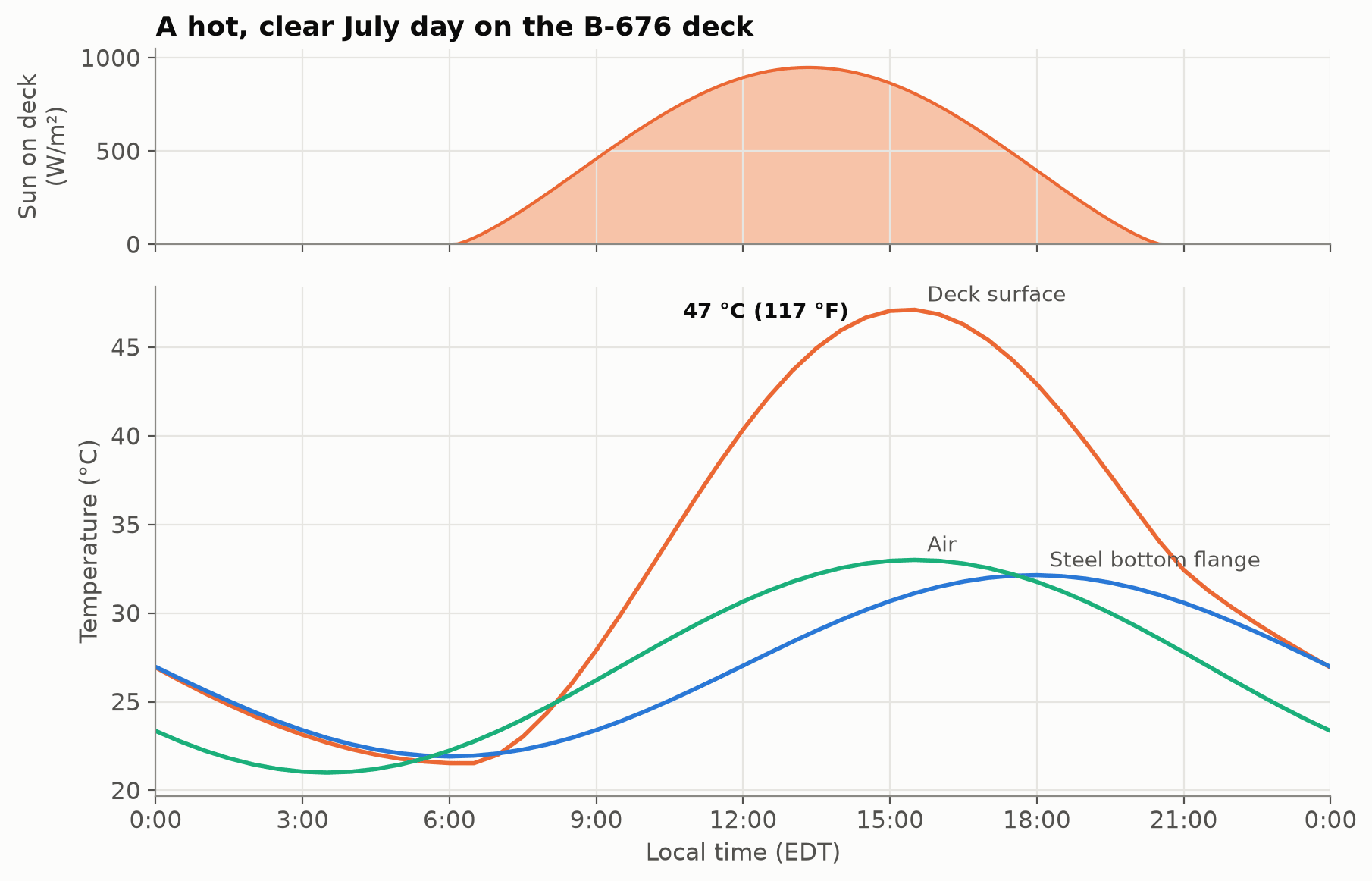A hot, clear July day: sun on the deck, and the deck surface, steel and air temperatures Figure 2. A hot, clear July day: the sun on the deck (top), and the deck surface, steel bottom flange and air temperatures (bottom).

The deck surface reaches 47 °C (117 °F) at 3:30 pm, about 14 °C above the air. The steel girders sit in shade under the deck and barely notice: they track the air temperature with a lag of about two hours.

That contrast is what matters structurally. A hot deck on cool steel is a temperature gradient: the top of the composite section wants to grow more than the bottom.

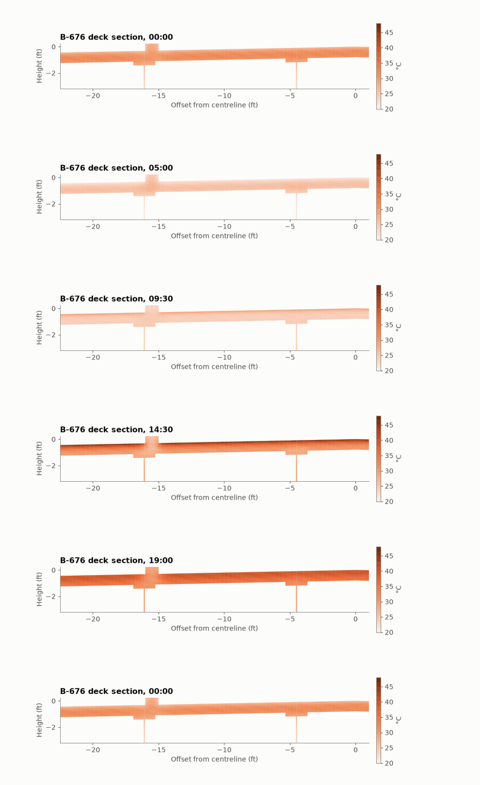Animation of the deck section through 24 hours Figure 3. The deck section through 24 hours.

The AASHTO LRFD specification (3.12.3) gives a design gradient for exactly this. Zone 2 is 46 °F at the top, dropping to 12 °F four inches down and to zero a foot below the surface.

The simulated peak gradient is 13.3 °C (24 °F), about 52% of the zone 2 design value. That’s what you’d hope to see: the code envelope covers rarer and harsher days than one clear July afternoon.

There’s also no real night-time reversal on a summer night. The thin steel cools with the air while the deck holds its heat, so the deck surface never gets more than a fraction of a degree colder than the girders. The code’s negative gradient belongs to cold, clear winter nights.

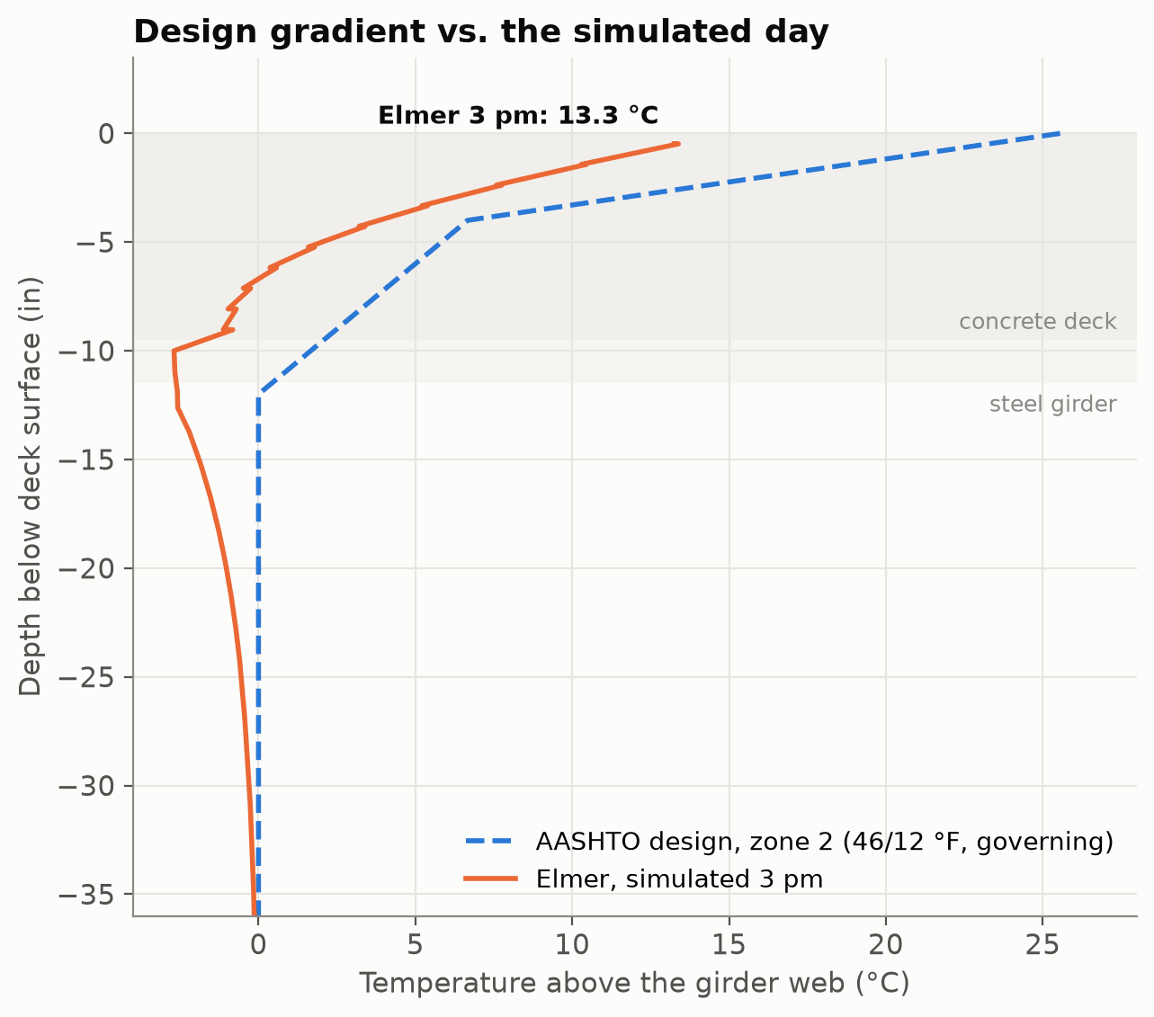Simulated gradient against the AASHTO zone 2 design gradient Figure 4. The simulated 3 pm gradient against the AASHTO zone 2 design gradient.

Shadows, and the girder that cooks at sunset

The first version of the thermal model treated the deck as a flat plate under the sun. Real bridges have parapets, rails and an orientation, so the second version added them:

Geometry: the 2% crown, the raised sidewalk, both parapets and the median rail.
The sun’s actual path: for this latitude, this date and this bridge’s N 40.9° E alignment.
Shadows: the parapets and median rail cast shadows whose width changes through the day.
Fascia girders: the outside girders catch direct sun on their outer webs, below the shadow line of the deck overhang.

Elmer doesn’t do ray tracing in this kind of model. Instead, the sun position, shadow edges and overhang shadow were written as small functions in Elmer’s built-in expression language (MATC) and evaluated at every boundary point and time step. The same geometry was reproduced in Python to draw the shadow map.

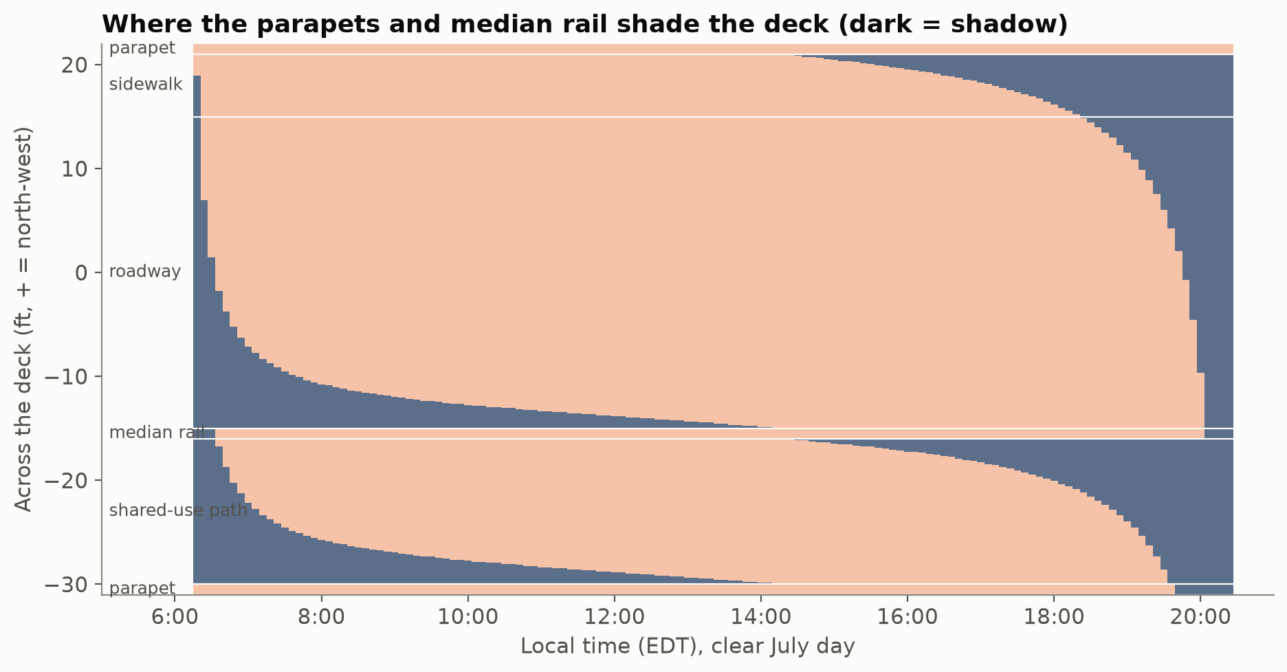Figure 5. Where the parapets and median rail shade the deck through the day (dark = shadow).

The pattern is easy to read once you see it:

Early morning: the sun rises in the east-north-east, about 20° off the bridge axis on the south-east side. The median rail and the south-east parapet throw long shadows across the roadway and the path.
By 8 am: those shadows have shrunk to a few feet.
From about 2:30 pm: the north-west parapet’s shadow starts creeping across the sidewalk. By sunset it covers the whole roadway.

The bigger surprise is the fascia girders:

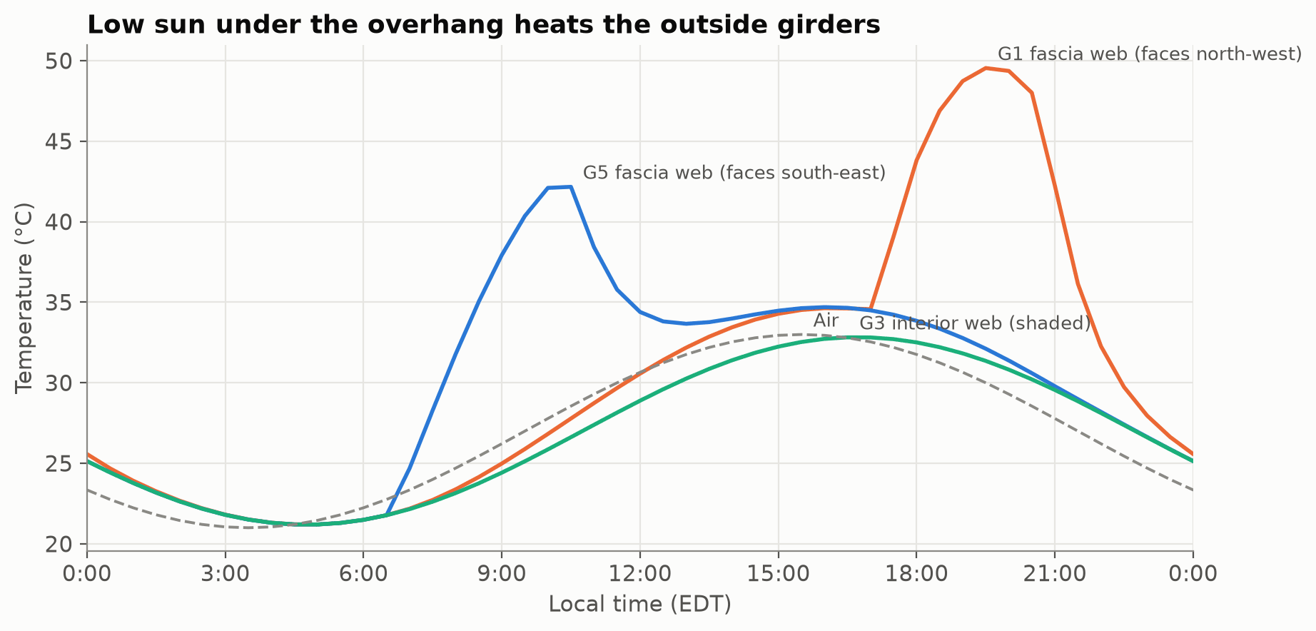Figure 6. Low sun under the overhang heats the outside girders, while the interior girder stays in shade.

North-west fascia (G1): in the early evening the sun is low in the west-north-west, nearly face-on to this web, and gets under the 3.3-ft deck overhang. The web passes 45 °C by 6:20 pm and peaks near 50 °C around 7:30 pm, as much as 18 °C hotter than the shaded interior girders.
South-east fascia (G5): gets the same treatment in the morning, peaking at about 42 °C at 10 am.

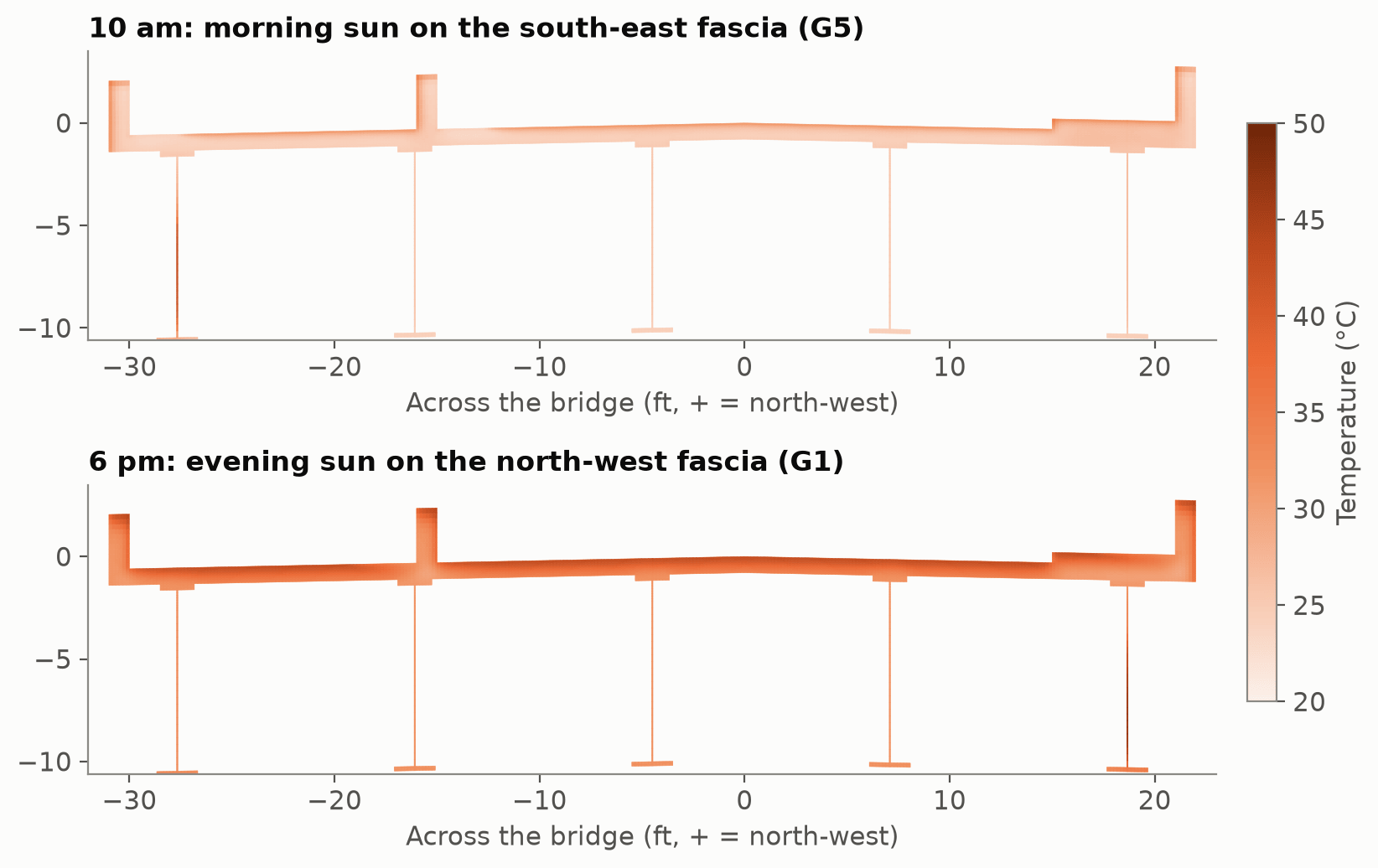Figure 7. Section temperatures at 10 am (sun on the south-east fascia) and 6 pm (sun on the north-west fascia).

This is the kind of effect a girder-line design approach can’t see. The cross-section now has a temperature that varies across the width as well as through the depth, and the hot outside girder wants to bow sideways.

From temperature to stress, with a check at every step

Before going 3D, the structure was modeled as a single interior girder line in 2D:

the composite section is represented as layers in plane stress;
each layer’s stiffness and mass are scaled by its real width;
quadratic elements are used throughout.

This model has one job: to be checkable. A continuous-beam calculation done independently in Python gives the same quantities, so every Elmer result can be compared with something.

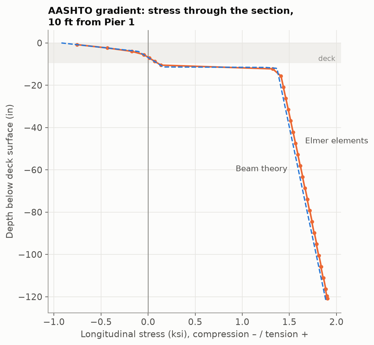Stress through the depth near Pier 1 under the AASHTO gradient: Elmer elements vs beam theory Figure 8. Stress through the depth 10 ft from Pier 1 under the AASHTO gradient: Elmer elements against beam theory.

When the two agreed, it meant something:

Quantity	Elmer against beam theory
Dead-load reactions	within 0.1%
Dead-load deflection	14.8 in against 14.5 in (the difference is shear deformation, which beam theory ignores)
Thermal-gradient bearing reactions	within 1.5%
Deck stress at the top surface	−0.92 ksi in both

When they disagreed, it meant a bug. The first versions disagreed in four different ways, and each disagreement turned out to be a modeling error rather than physics:

Over-restrained bearings. The bearings were modeled as 12-inch pads restrained at three nodes, which clamped the girder ends against rotation. Dead-load deflection came out 13% too stiff.
Longitudinal restraint on a whole pad. Fixing the whole pad longitudinally stopped the steel flange’s own thermal expansion and created a fake local stress.
Averaged stresses. Elmer averages stresses at nodes, so stresses at the steel–concrete interfaces mixed two very different materials. The result was 8 ksi “stripes” in the stress plots. Recomputing stresses inside each element fixed it.
Dead load on the wrong section. It was first applied to the composite section. On a real bridge the wet concrete is carried by the steel alone, so it belongs on the non-composite girder, which roughly doubles the deflection.

None of these crashed or produced a warning. All four produced smooth, reasonable-looking plots.

Going 3D: the deck curls across its width

The 3D model covers the full width:

Structure: deck, haunches, all five girders, the crown and the 10° skew.
Cross-frames: X cross-frames (pairs of L4×4×½ angles) are represented as equivalent shear panels between the girder webs. The panels’ stiffness is matched to the racking stiffness of the real bracing. They sit about every 20–24 ft and next to every bearing line.
Bearings: single points. Pier 1 is fixed longitudinally and the centre girder is guided laterally.

Under the AASHTO design gradient, the superstructure bows up in the end spans, by up to 0.58 inches, and pushes down in the middle span:

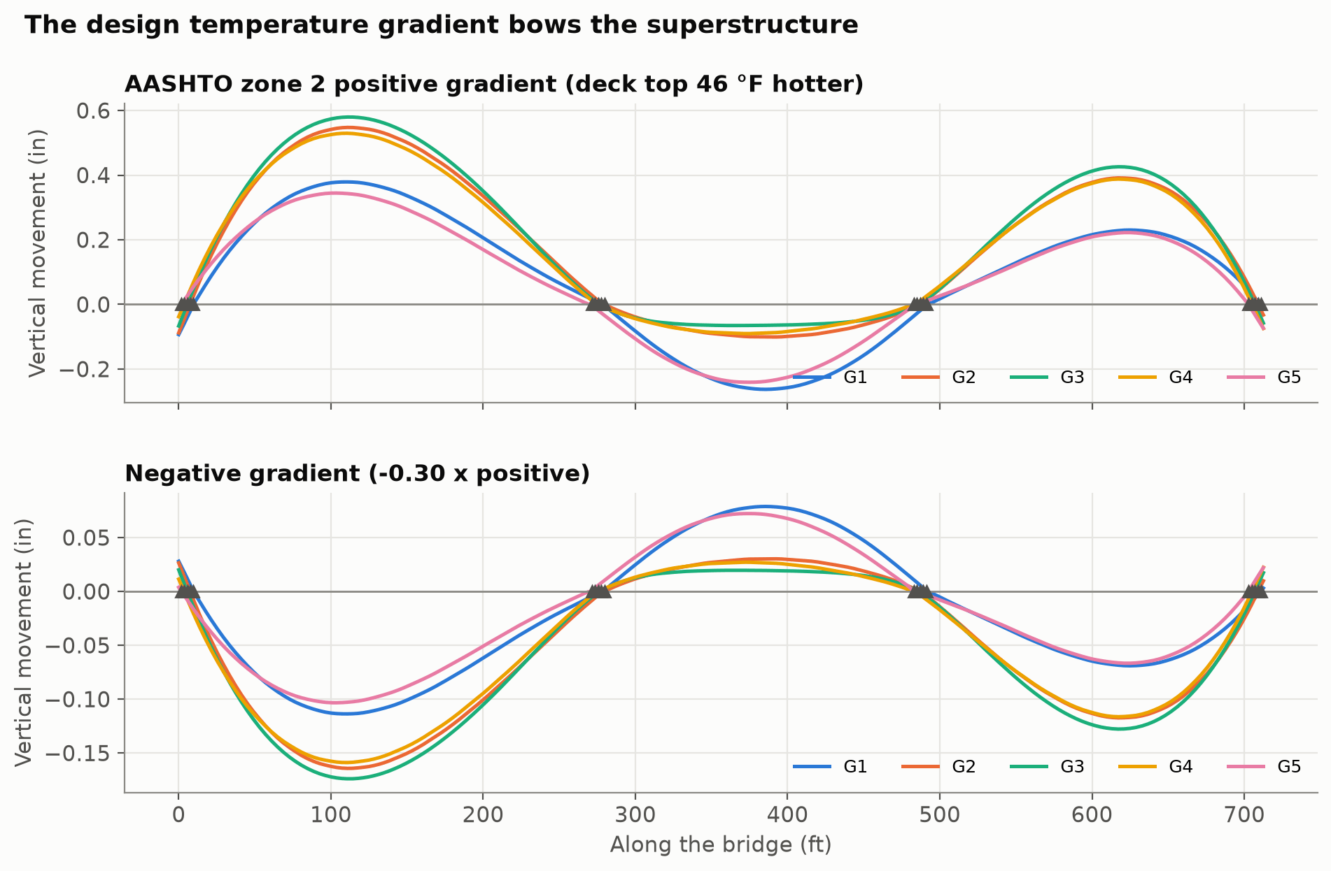The design temperature gradient bows the superstructure (all five girders) Figure 9. The AASHTO positive and negative design gradients bow the superstructure (all five girders).

A girder-line model sees exactly that, and says each bearing picks up or sheds about 8 kips. The 3D model sees something else as well.

The deck also curls across its width. A slab that’s hot on top doesn’t just want to arch along the span. It wants to dome in both directions.

At each pier, the bearings have to flatten that dome. The exterior bearings press down harder by about +100 kips, while the interior ones are relieved by up to −94 kips. Yet the total at each support line still matches five times the girder-line answer to within 2%.

Because this was new and large, it was tested before it was believed:

refining the deck mesh changed it by 2–5%;
changing the lateral restraint changed it by about 10%;
a hand estimate from the deck’s thermal moment gives the same order of magnitude.

The answer the engineer needed is reassuring: no bearing comes close to lifting off. Under dead load plus the worst thermal or shrinkage case, the lightest bearing still carries at least 163 kips.

The sunny-day simulation then drove the 3D model directly. The full 3D heat analysis was run on the same mesh and fed into the stress analysis at 3:20 pm and 6:20 pm. Its temperatures match the 2D thermal model to within about 0.5 °C at every check point and time.

In the evening case, the sun-baked north-west fascia makes the response visibly asymmetric:

at Pier 1, G1’s bearing changes by +93 kips while G5’s changes by +61 kips;
G1’s bottom flange moves sideways about a tenth of an inch.

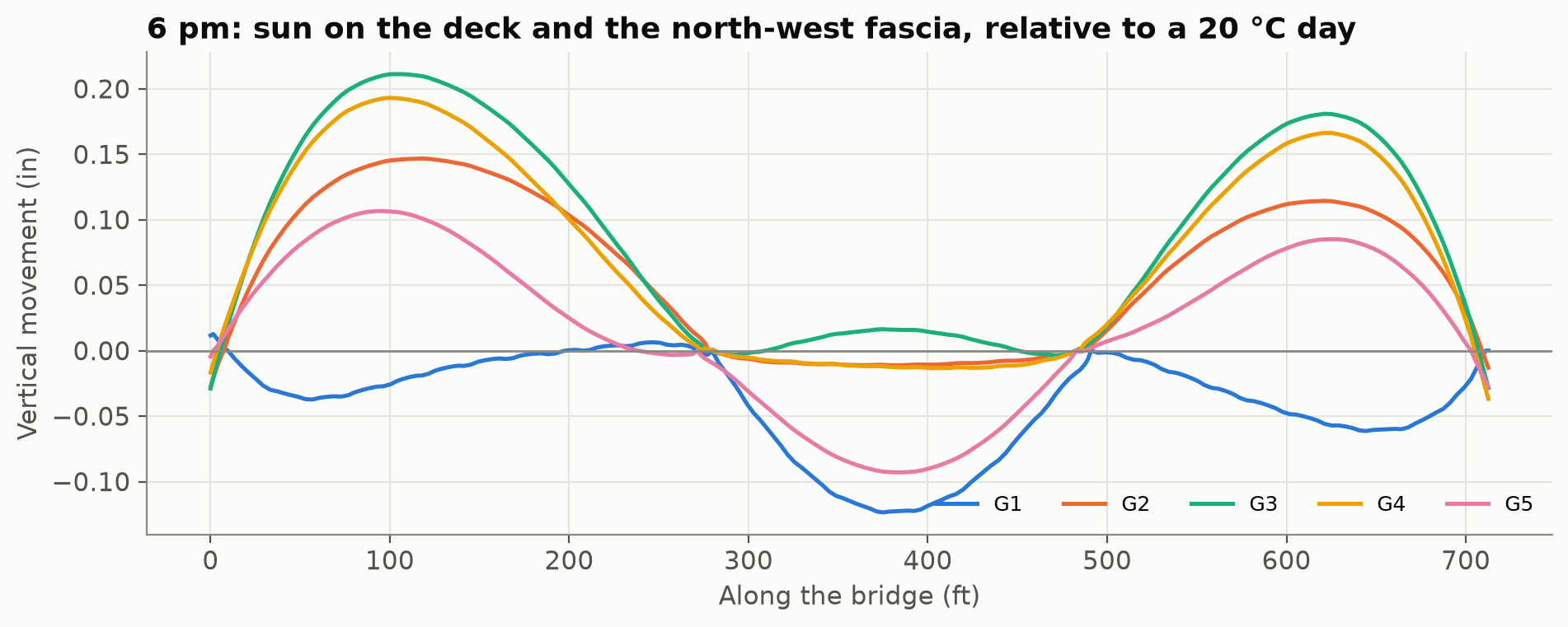6 pm: sun on the deck and the north-west fascia Figure 10. Vertical movement at 6 pm, with sun on the deck and the north-west fascia, relative to a uniform 20 °C day. The hot G1 fascia moves differently from the other four girders.

Building the camber

Steel bridges are built in stages. The deflection at each stage has to be built into the girders as camber, so the finished deck comes out at the right grade:

Stage 1: the steel and the wet deck are carried by the bare girders.
Stage 2: parapets, sidewalk, median rail and future overlay go on the hardened, composite deck. Long-term loads use the creep-reduced concrete stiffness.
Long term: the deck shrinks.

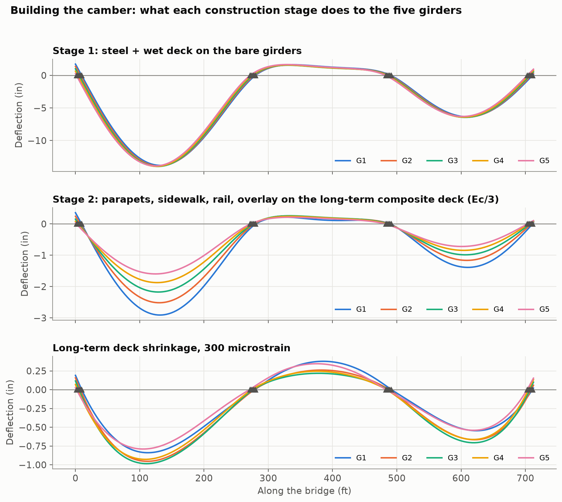Figure 11. What each construction stage does to the five girders.

For the interior girder in span 1 that adds up to:

Stage	Deflection
Steel + wet deck	14.0 in
Superimposed dead load	2.2 in
Shrinkage	1.0 in
Total camber	about 17 in

The short middle span does the opposite during the deck pour. Its long neighbours rotate it over the piers, and it rises about 1.6 inches. A fabricator who missed that would build the wrong camber into the middle span.

The stage-2 plot also shows the asymmetry of the cross-section. The north-west side carries the heavier parapet and the sidewalk, so G1 deflects 2.9 inches against 1.6 inches for G5.

The skew shows up in the bearing reactions too. Dead load concentrates toward the obtuse corners of a skewed span. G1’s bearing at the first abutment carries 328 kips, against 283 kips for the same bridge on square supports, a 16% increase.

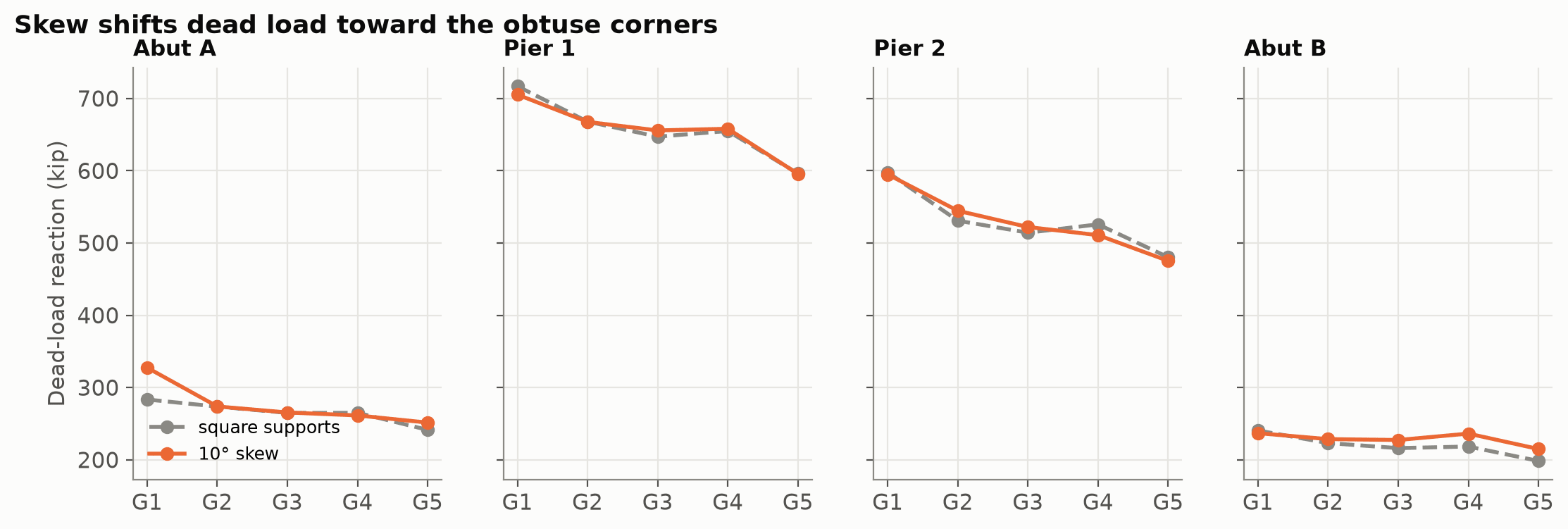Skew shifts dead load toward the obtuse corners Figure 12. Dead-load bearing reactions on square and 10° skewed supports. Skew shifts load toward the obtuse corners.

Trucks, everywhere

Design codes don’t ask “what does one truck do?” They ask “what is the worst a girder can see from any legal arrangement of trucks?” AASHTO answers that with distribution factors: formulas that say how many lanes of load each girder must be designed for.

The 3D model answers it directly. One HL-93 design truck (with 33% impact) was placed at seven transverse positions across the roadway, in two different spans. That’s 14 full 3D analyses.

Each girder’s moment was recovered from its bottom-flange stress and section modulus. The results were then combined by superposition into every legal case:

one truck, anywhere, with AASHTO’s 1.2 multiple-presence factor;
two trucks side by side, at least 10 feet apart.

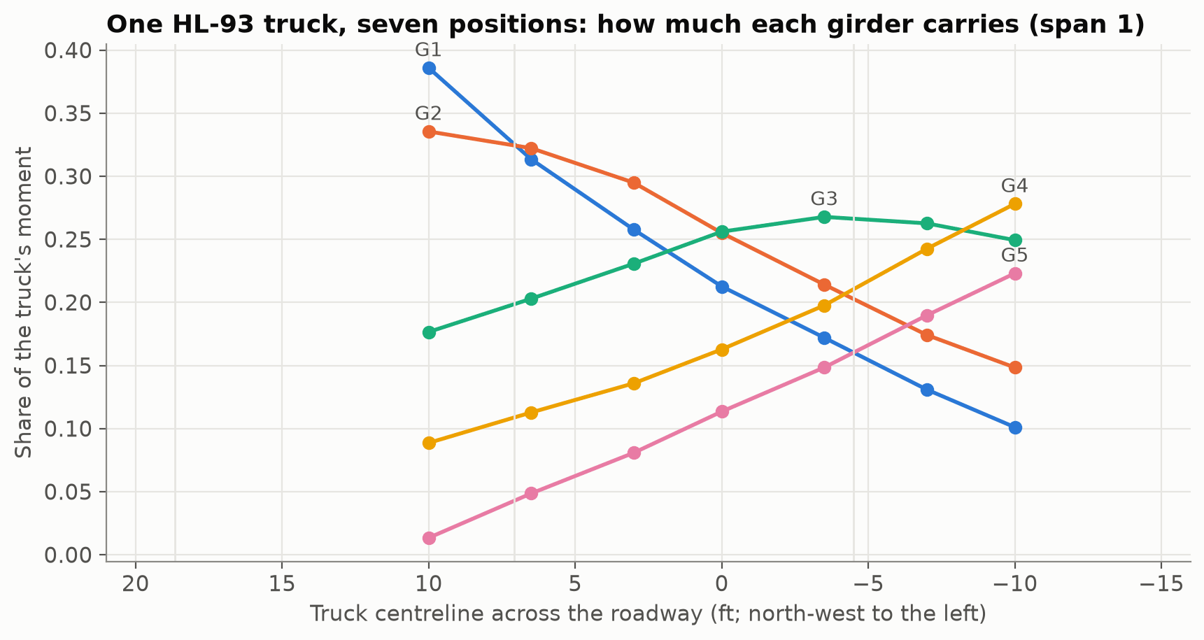One truck, seven positions: how much of the truck each girder carries Figure 13. One truck at seven positions across span 1: the share of the truck’s moment that each girder carries.

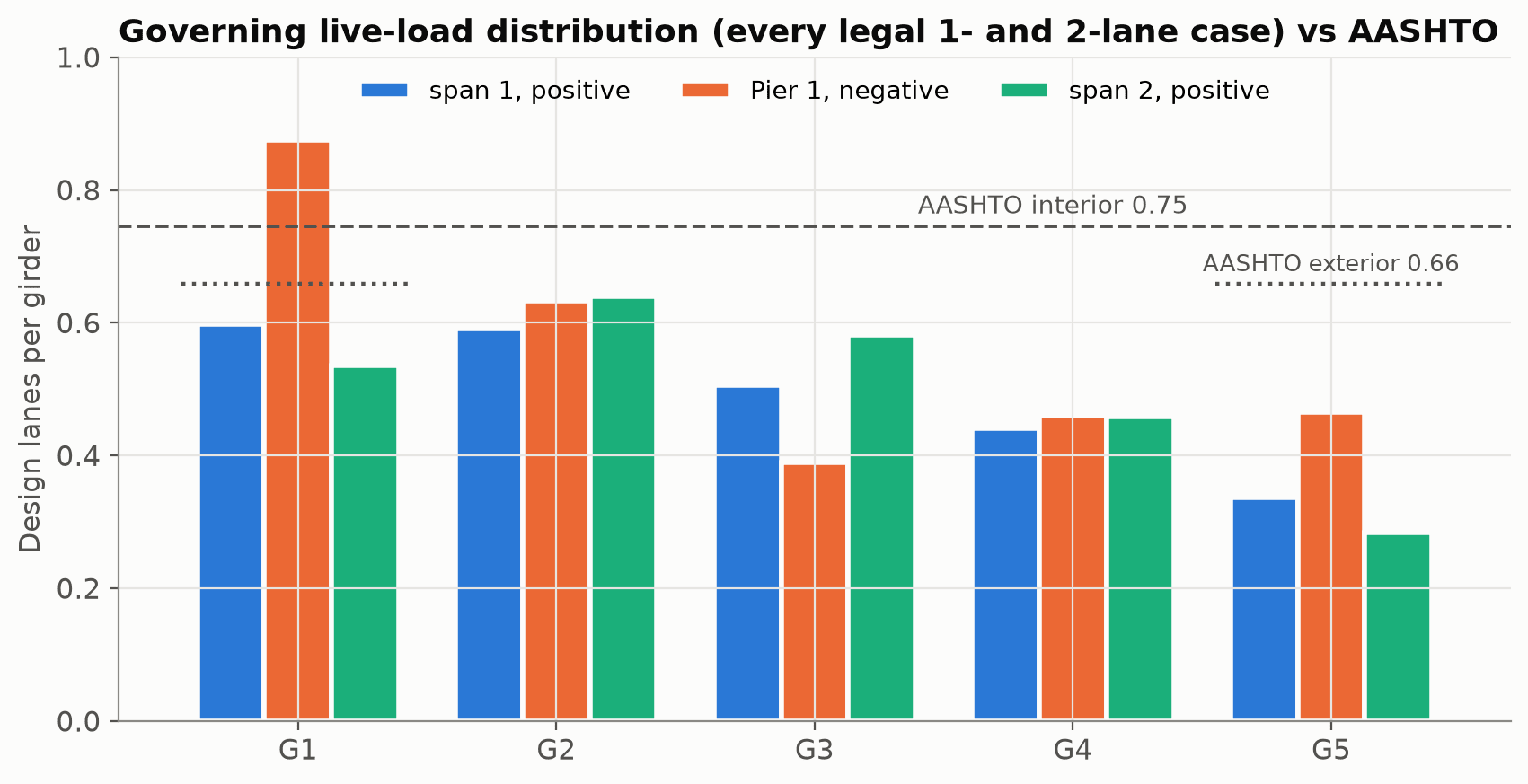Figure 14. Governing live-load distribution from every legal one- and two-lane case, compared with the AASHTO factors.

For positive moment, the AASHTO formulas are conservative here:

Interior girders: the worst carries 0.59–0.64 lanes in the 3D model, against 0.75–0.80 from the formula.
Exterior girder: 0.60 against 0.66 from AASHTO’s rigid-body check.

Near the skewed pier, though, the exterior girder’s share of negative moment comes out at 0.88, above the AASHTO exterior value. That result sits right next to a skewed bearing and the support cross-frames, where local effects mix in. It’s flagged here as something a designer would confirm with a finer model, not as a finding.

Live-load deflection passes comfortably:

averaged over the girders, the governing AASHTO combination (25% of the truck plus the lane load) deflects span 1 by about 1.2 in, and the most-loaded girder by about 1.6–1.7 in;
the limit for a bridge with pedestrians (L/1000) is 3.24 in.

The truck sweep also measured the cross-frames:

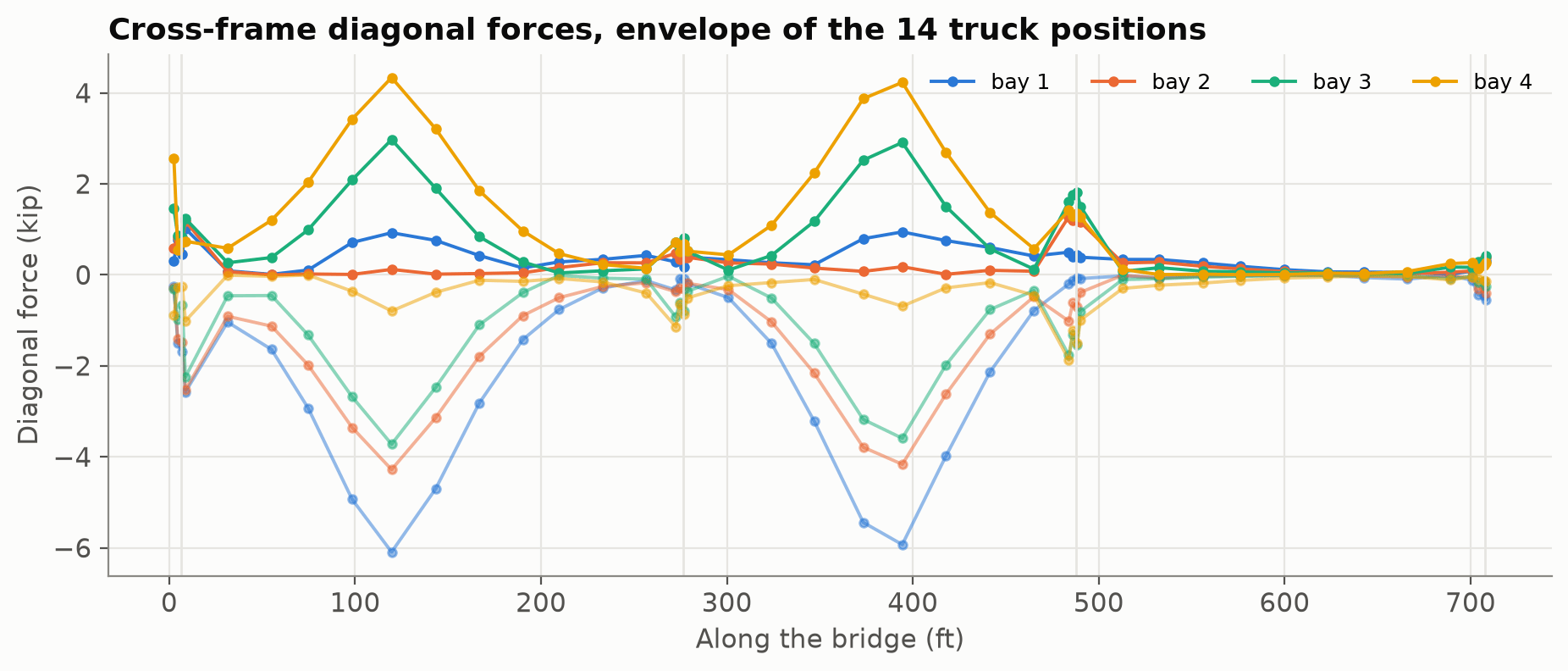Cross-frame diagonal forces, envelope of the 14 truck positions Figure 15. Cross-frame diagonal forces in each bay: the envelope of the 14 truck positions.

The most heavily loaded diagonals see about 6 kips of compression under a design truck, and swing through about 7 kips as the truck moves across. For fatigue, the stress range in an L4×4×½ diagonal is 2.8 ksi. That clears the 4.5 ksi infinite-life threshold for a Category E connection, but not the 2.6 ksi threshold for Category E′, the classification for an angle welded on one leg.

In other words, the connection detail decides it. That is precisely the sort of thing skewed steel bridges are known for, and it only showed up once the model was refined (more on that below).

How it vibrates

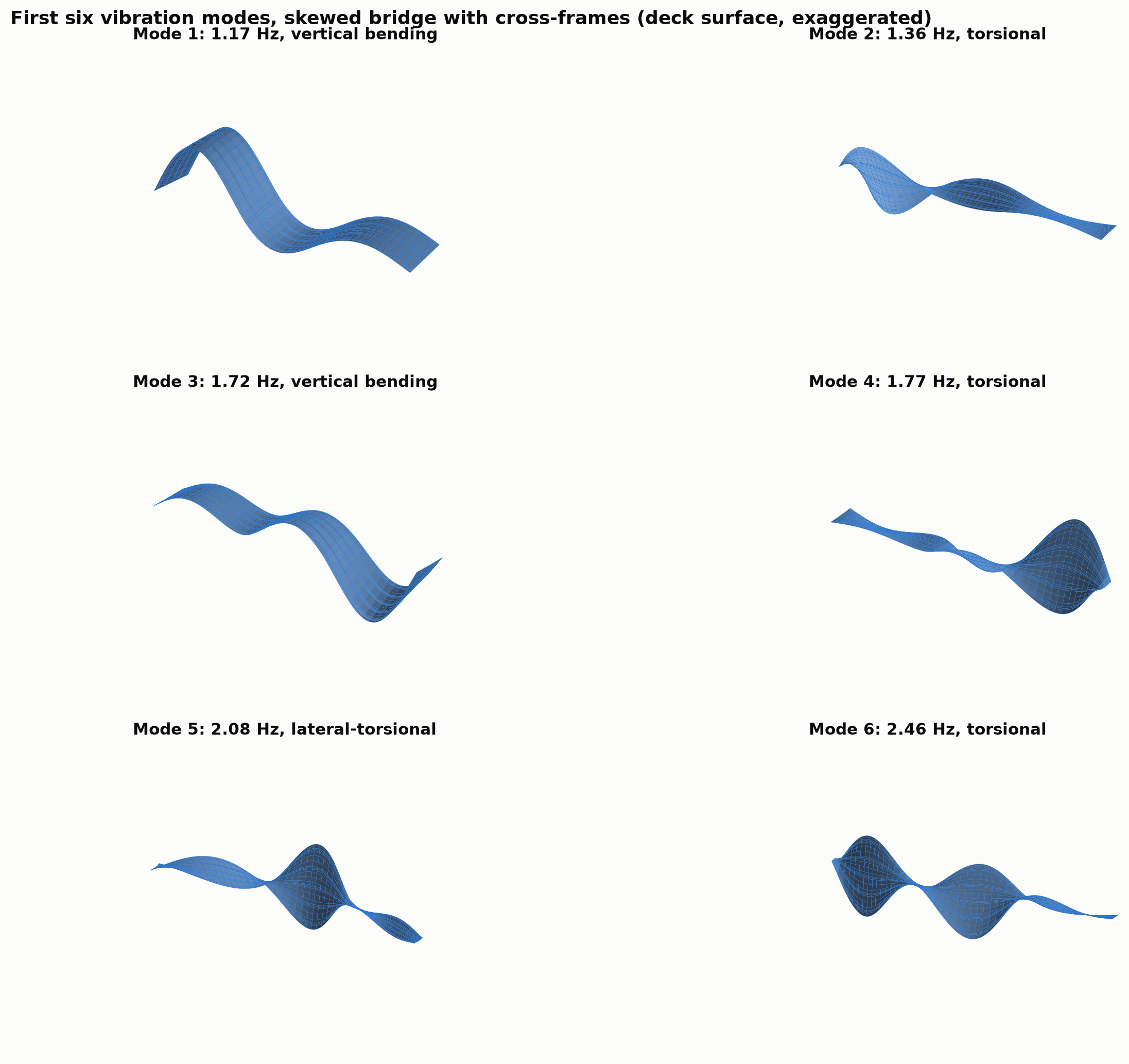Figure 16. The first six vibration modes of the superstructure (deck surface, exaggerated).

The first vertical bending mode is at 1.17 Hz. The first torsional mode follows close behind at 1.36 Hz. After that come more bending and torsion modes, and a lateral-torsional sway at about 2.1 Hz.

Adding the cross-frames raised the first torsional frequency, which is exactly what cross-frames are for. The vertical frequency agrees with the 2D girder line once the mass of the parapets and sidewalk is accounted for.

Getting these numbers right took one more catch. The equivalent cross-frame panels had been given zero density. That made the mass matrix singular, and the eigenvalue solver returned frequencies of 20 to 100 Hz without any warning. Giving the panels the real mass of the steel angles brought the answers back into line.

The code check: the BIM girder isn’t a designed girder

The last step was an AASHTO LRFD check of the girders, done the way most designers do it:

a line-girder analysis with influence lines;
moving HL-93 trucks and tandems, the lane load, and the 90% two-truck rule for negative moment;
the fatigue truck;
section properties for the steel-only, long-term composite, short-term composite and negative-moment sections.

The checks themselves:

Strength I: positive and negative flexure, and shear.
Service II.
Constructibility during the deck pour: the top flange is braced only by the cross-frames, and the web can bend-buckle.
Fatigue I: at the cross-frame connection plates.

The girder in the Revit model had constant flanges, a 20 × 1.5 in top and a 24 × 2.5 in bottom, chosen for a visualization model. The code check is blunt about it:

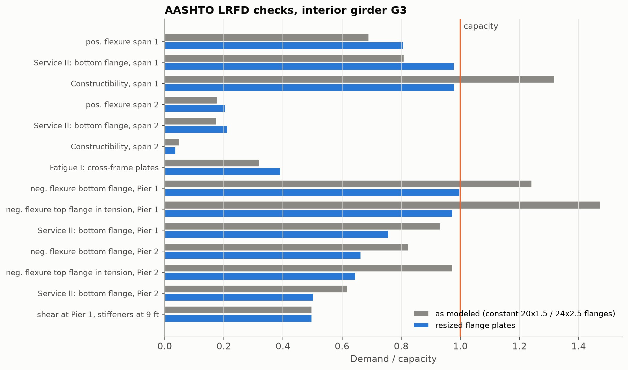AASHTO LRFD checks for the interior girder: as modeled vs resized flange plates Figure 17. AASHTO LRFD checks for interior girder G3: the flanges as modeled in Revit against the resized flange plates.

Positive flexure and fatigue: fine (0.69 and 0.32).
The deck pour: fails at 1.32. The deep, slender web bend-buckles under the stress of the wet concrete before the top flange yields.
Over Pier 1: the bottom flange is at 1.24 and the top flange, in tension, at 1.47.
Shear: an unstiffened web fails at 1.72. Transverse stiffeners at 9 ft bring that to 0.50.
Without the intermediate cross-frames: the compression flange would be unbraced for the full 270-ft span during the pour, and the check exceeds capacity by a factor of about seventy. Cross-frames aren’t decoration.

So the checker took the next step a designer would. It searched standard plate sizes for the lightest flanges that pass every check: one section for the positive-moment regions, and a heavier one over the piers.

With AASHTO’s distribution factors, the interior girder needs:

a 24 × 1.5 top and a 22 × 2.0 bottom flange in the spans;
a 20 × 3.0 top and a 26 × 2.75 bottom flange over the piers.

Then the same search was run with the distribution factors from the 3D model:

Girder	Region	Flange area, AASHTO factors	Flange area, 3D factors	Change
Interior G3	spans	80 in²	71 in²	−11%
Interior G3	piers	132 in²	104 in²	−21%
Exterior G1	piers	111 in²	125 in²	+13%

That is a nuanced answer, and an honest one. Refined analysis isn’t a free lunch: it takes steel out of some members and puts it into others. Here it puts steel into the exterior girder over the skewed pier, the same place the 3D model flagged earlier.

What it took

The “AI runs an FE model” headline hides how many ways an analysis can be confidently wrong. Here is the full list of errors in this study that produced plausible output and were caught only by an explicit check:

Bearing pads that clamped the girder ends (dead load 13% too stiff).
A longitudinal restraint that stopped the flange’s own thermal expansion.
Nodal stress averaging across materials (fake 8 ksi stripes).
Dead load on the composite instead of the steel section.
A missing feet-to-metres factor that made the wet-deck load 3.28 times too large. With the steel weight unaffected, the reactions summed to 17,062 kips instead of 6,611.
Point loads written in a form that, in 3D, silently applied nothing (all reactions zero).
A single laterally guided girder that let the cross-section rack, producing a spurious 0.63 Hz “lateral” mode.
A mesh-cleanup command that silently deleted every bearing and wheel-load point.
Zero-density cross-frame panels that wrecked the vibration analysis.
An off-by-one in how Elmer numbers its saved time steps, which put the “3 pm” restart at 12:20 pm.
Steel faces next to the cross-frame panels that never became thermal boundaries, so the girder webs were thermally insulated and ran up to 10 °C too hot.

Every one of them was caught by comparing against something independent:

the reaction sum against the hand-computed load;
the deflection against beam theory;
the 3D heat field against the 2D one;
frequencies against an earlier model;
a simple question: “does that number make physical sense?”

The agent wrote and ran those checks. But a person with engineering judgment decided what had to be checked and what “close enough” meant, and signs the drawings.

There was also a hardware lesson. The stock Windows build of Elmer solves with a single-threaded direct solver limited to 32-bit integer indexing. That capped the 3D model at about 82,000 nodes, which forced simple 8-node elements, and running cases in parallel helped only 1.4×.

Partway through, the study switched to Elmer’s MPI build with the MUMPS solver:

the same 3D model solved in 6 seconds instead of 80, with identical results;
meshes of over 150,000 nodes became routine;
quadratic elements became affordable.

The quadratic elements showed that the production linear mesh had been 3–5% too stiff, and its cross-frame forces 60% too low. That is why the Category E′ fatigue question surfaced only at the end.

The honest limits

Weather: one synthetic clear July day, not measured weather, and a bare concrete deck with no overlay.
Live load: two longitudinal truck positions per span and seven transverse ones. A design would use full influence surfaces and moving loads in 3D.
Cross-frames: equivalent shear panels rather than individual members. The diagonal forces are recovered from panel shear.
Code checks: on a line-girder model with prismatic stiffness. A real design would vary plate sizes along the girder and re-analyse.
Not modeled: pier and abutment flexibility, bearing stiffness, and the deck pour sequence.
Material properties: typical values, not taken from plans.

To repeat the disclaimer: these simulations are for demonstration and education only. They are not engineering work stamped or sealed by a licensed Professional Engineer, and they must not be used to design, build, rate or evaluate any real structure.

The steam shovel, again

The analogy from The Steam Shovel Moment and Steam Shovels for Design Engineers holds up even better for analysis than for drafting. The steam shovel didn’t decide where the canal went. It moved more earth than any crew with hand shovels could, and that freed the engineers to think about the hard parts: drainage, slides, sequence.

In this study the agent did the earth-moving:

meshes, input files, dozens of runs, post-processing and plots;
an AASHTO checker and a plate-sizing search;
the 3D heat-to-stress coupling;
a migration to a faster solver build halfway through.

At engineering billing rates, a human team would have spent weeks on that.

What it couldn’t do on its own was know which answers to distrust. Eleven times, the right response to a smooth, confident plot was “that can’t be right,” followed by an independent check. That instinct, and the professional responsibility that comes with it, is the part of the job that stays with the engineer.

Built with Claude Code driving Elmer FEM 26.2 on a Windows workstation through custom Python helpers and a reusable Elmer skill.

Sources and further reading

TeraContext.AI, Steam Shovels for Design Engineers (November 7, 2026), the Civil 3D, Revit and Navisworks work on the same bridge, and The Steam Shovel Moment for Civil Engineering Drafting (October 8, 2026).
Elmer FEM (CSC – IT Center for Science), its source repository, and the 26.2 release.
AASHTO LRFD Bridge Design Specifications: 3.6 (live load), 3.12.3 (temperature gradient), 4.6.2.2 (distribution factors), 5.4.2.4 (concrete modulus), 6.6.1 (fatigue), 6.10 (I-section flexural members).
MUMPS, the parallel sparse direct solver used in the final runs.